4 Aerial Cityscapes
Motivation
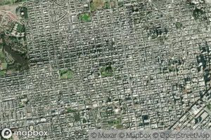
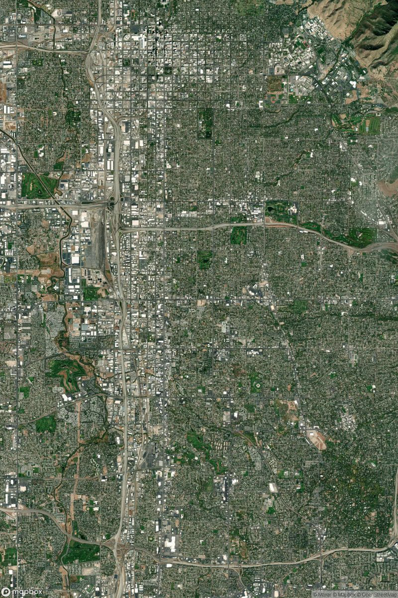
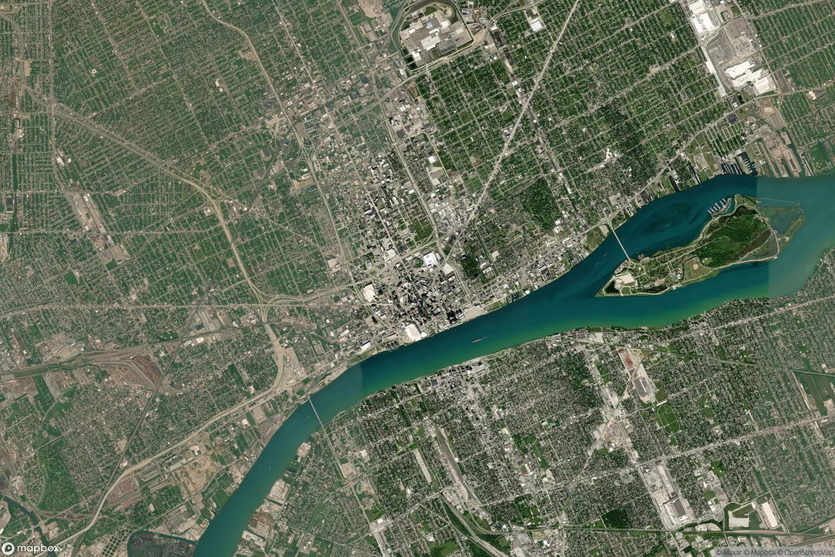
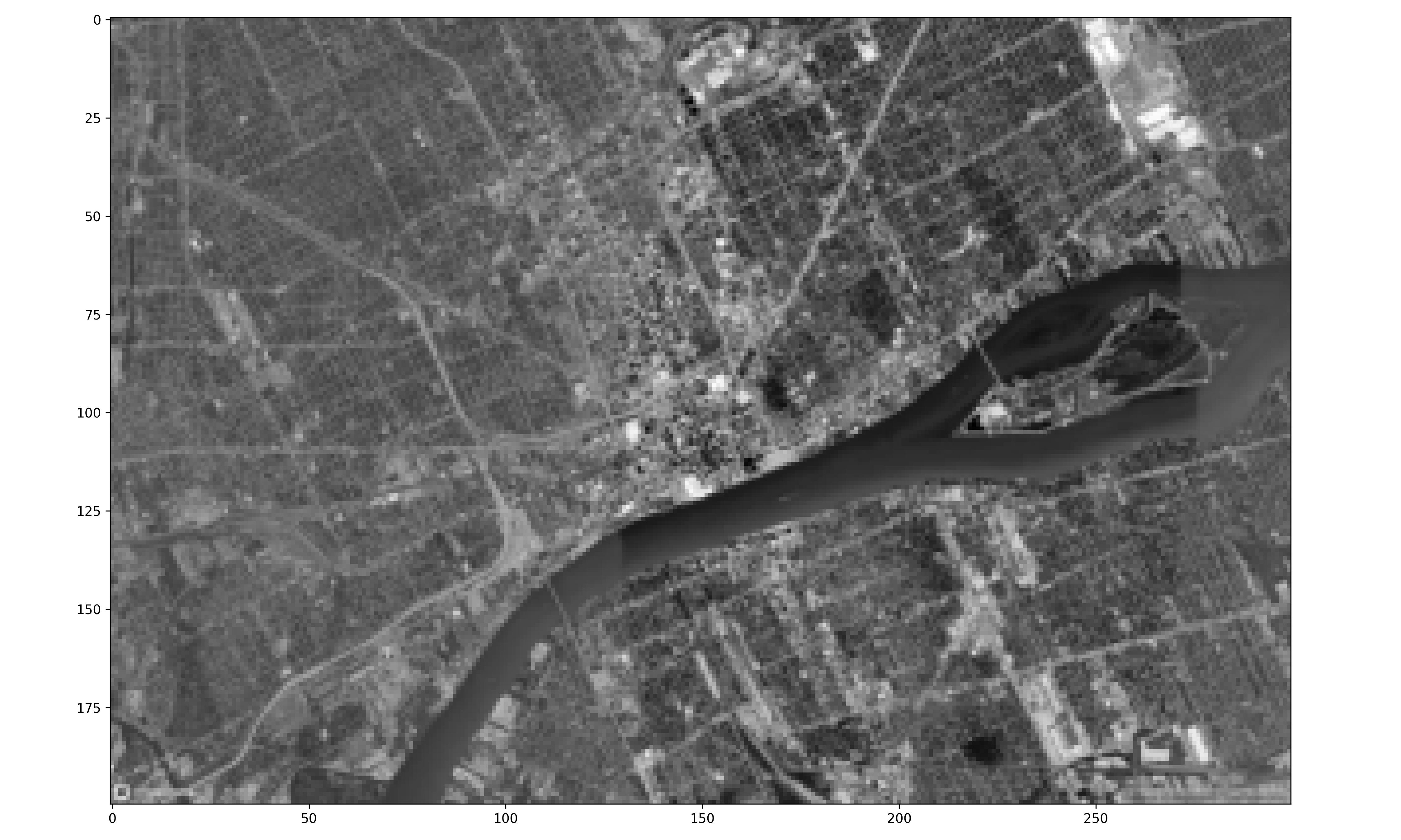
Download aerial cityscape images from Mapbox’s API of San Francisco, Salt Lake City, and Detroit to determine if the HOG algorithm is capable of identifying dominant angles of each city’s grid layout.
Load R Packages and Python Libraries
Load Python Libraries
# Load Python Libraries
import matplotlib.pyplot as plt
import pandas as pd
from skimage.io import imread, imshow
from skimage.transform import resize
from skimage.feature import hog
from skimage import data, exposure
import matplotlib.pyplot as plt
from skimage import io
from skimage import color
from skimage.transform import resize
import math
from skimage.feature import hog
import numpy as np
Download Aerial City Images from Mapbox
Download map of San Francisco, CA
Download map of Salt Lake City, UT
# Download map of Salt Lake City, UT
points_of_interest <- tibble::tibble(
  longitude = c(-112.065945, -111.853948,
                -111.852956, -112.023371),

  latitude = c(40.794275, 40.791516,
               40.502308, 40.502308)
  )

prepped_pois <- prep_overlay_markers(
  data = points_of_interest,
  marker_type = "pin-l",
  label = 1:4,
  color = "#fff",
)

map <- static_mapbox(
  access_token = key,
  style_url = "mapbox://styles/mapbox/satellite-v9",
  width = 800,
  height = 1200,
  image = T,
  latitude = 40.7,
  longitude = -111.876183, zoom = 12
)

magick::image_write(map, "images/salt_lake_city_zoom_12.png")
Download map of Detroit, MI
Collect HOG Features for Aerial Cityscapes
Rescale and convert each image to grayscale. Then iterate through the list of images and collect gradient magnitudes and angles.
# List for storing images
img_list = []
# SF aerial
img_list.append(color.rgb2gray(
io.imread("images/san_francisco_scale_zoom_12.png")))
# Salt Lake City Aerial
img_list.append(color.rgb2gray(
io.imread("images/salt_lake_city_zoom_12.png")))
# Detroit Aerial
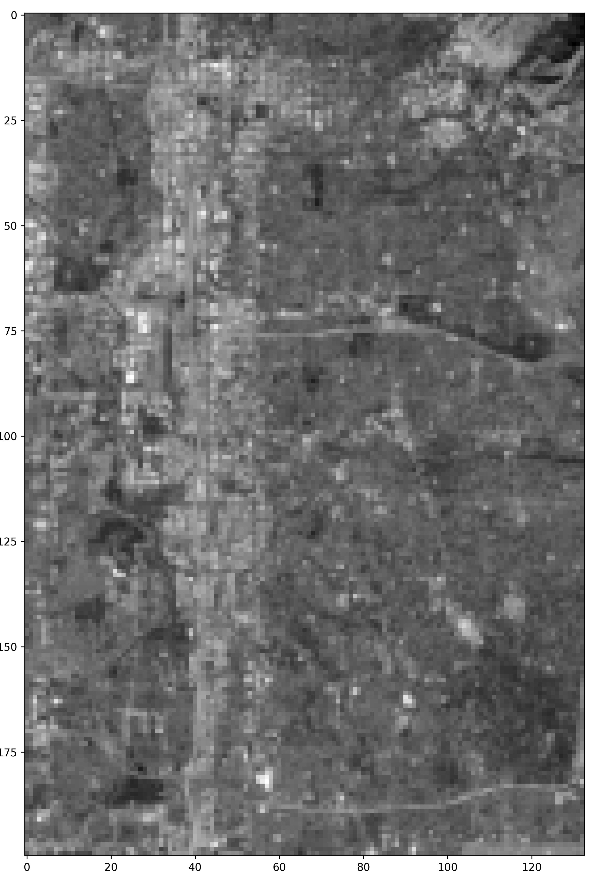
img_list.append(color.rgb2gray(io.imread("images/detroit_zoom_12.png")))
# List to store magnitudes for each image
mag_list = []
# List to store angles for each image
theta_list = []
for x in range(len(img_list)):
# Get image of interest
img = img_list[x]
rescaled_file_path = f"images/plots/aerial_cities/{x}.jpg"
# Determine aspect Ratio
aspect_ratio = img.shape[0] / img.shape[1]
print("Aspect Ratio:", aspect_ratio)
# Hard-Code height to 200 pixels
height = 200
# Calculate witdth to maintain same aspect ratio
width = int(height / aspect_ratio)
print("Resized Width:", width)
# Resize the image
resized_img = resize(img, (height, width))
# Replace the original image with the resized image
img_list[x] = resized_img
# if (x == 1):
# plot_width = 8
# plot_height = 15
# else:
# plot_width = 15
# plot_height = 9
#
# plt.figure(figsize=(plot_width, plot_height))
# plt.imshow(resized_img, cmap="gray")
# plt.axis("on")
# plt.tight_layout()
# plt.savefig(rescaled_file_path, dpi=300)
# plt.show()
# list for storing all magnitudes for image[x]
mag = []
# list for storing all angles for image[x]
theta = []
for i in range(height):
magnitudeArray = []
angleArray = []
for j in range(width):
if j - 1 < 0 or j + 1 >= width:
if j - 1 < 0:
Gx = resized_img[i][j + 1] - 0
elif j + 1 >= width:
Gx = 0 - resized_img[i][j - 1]
else:
Gx = resized_img[i][j + 1] - resized_img[i][j - 1]
if i - 1 < 0 or i + 1 >= height:
if i - 1 < 0:
Gy = 0 - resized_img[i + 1][j]
elif i + 1 >= height:
Gy = resized_img[i - 1][j] - 0
else:
Gy = resized_img[i + 1][j] - resized_img[i - 1][j]
magnitude = math.sqrt(pow(Gx, 2) + pow(Gy, 2))
magnitudeArray.append(round(magnitude, 9))
if Gx == 0:
angle = math.degrees(0.0)
else:
angle = math.degrees(math.atan(Gy / Gx))
if angle < 0:
angle += 180
angleArray.append(round(angle, 9))
mag.append(magnitudeArray)
theta.append(angleArray)
# add list of magnitudes to list[x]
mag_list.append(mag)
# add list of angles to angle list[x]
theta_list.append(theta)Aspect Ratio: 0.6666666666666666
Resized Width: 300
Aspect Ratio: 1.5
Resized Width: 133
Aspect Ratio: 0.6666666666666666
Resized Width: 300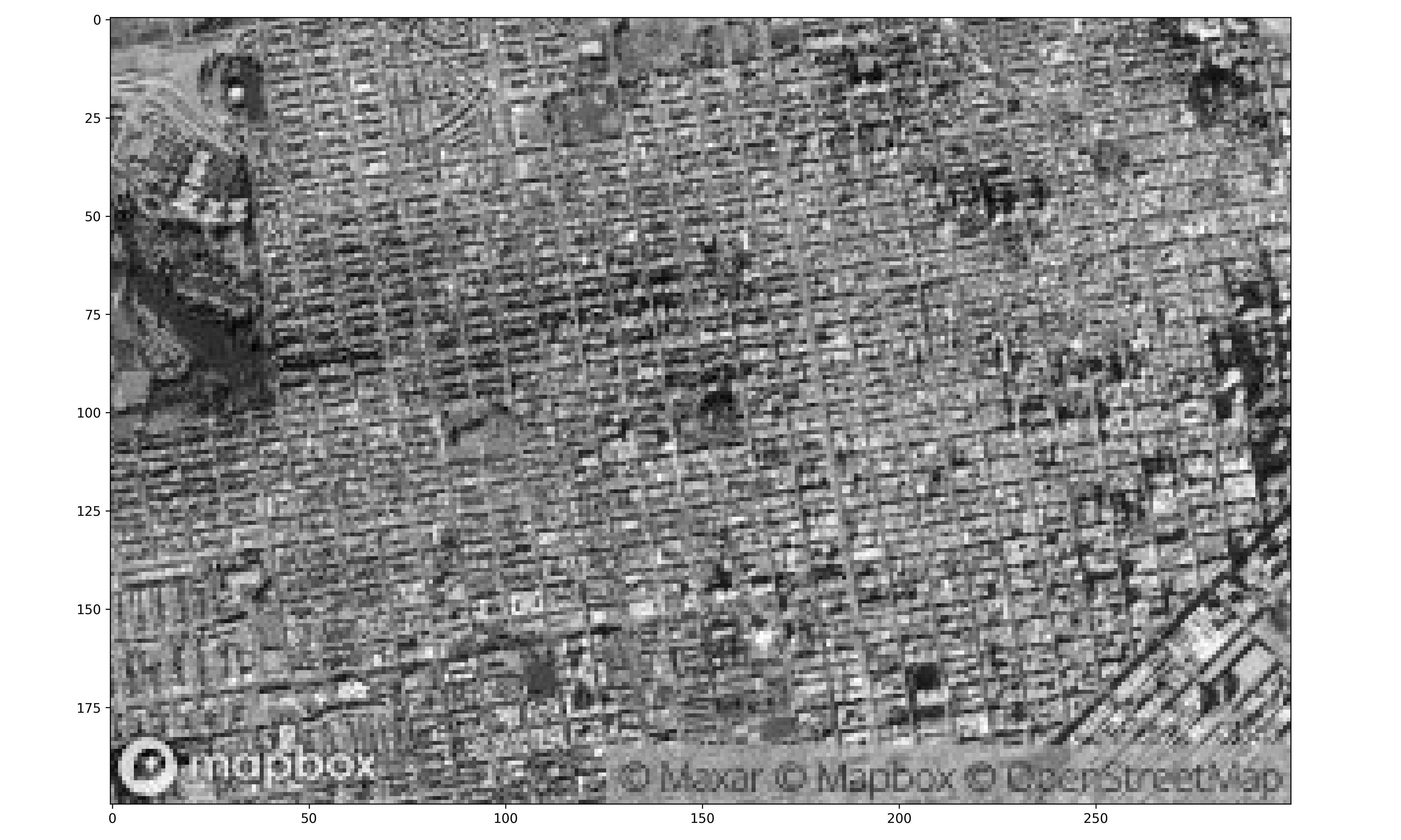
Extract Gradient Magnitudes and Angles from each Aerial Cityscape
Create arrays of gradient magnitudes and angles for each image
# San Francisco DF of gradient magnitudes and angles
mag_sf = np.array(mag_list[0])
theta_sf = np.array(theta_list[0])
# Salt Lake City DF of gradient magnitudes and angles
mag_salt_lake = np.array(mag_list[1])
theta_salt_lake = np.array(theta_list[1])
# Detorit DF of gradient magnitudes and angles
mag_detroit = np.array(mag_list[2])
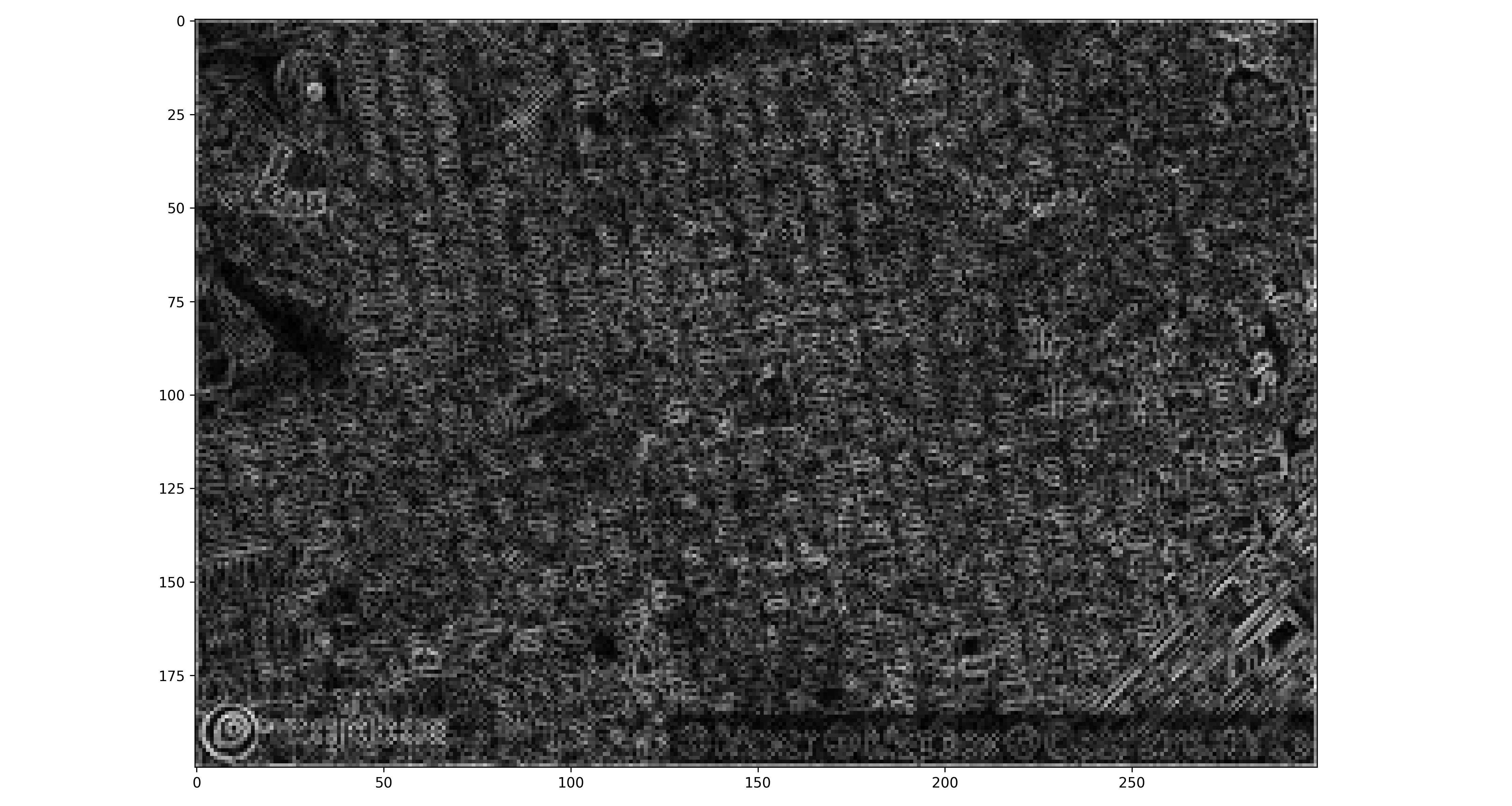
theta_detroit = np.array(theta_list[2])Plot Gradient Magnitudes as Image for each Aerial Cityscape
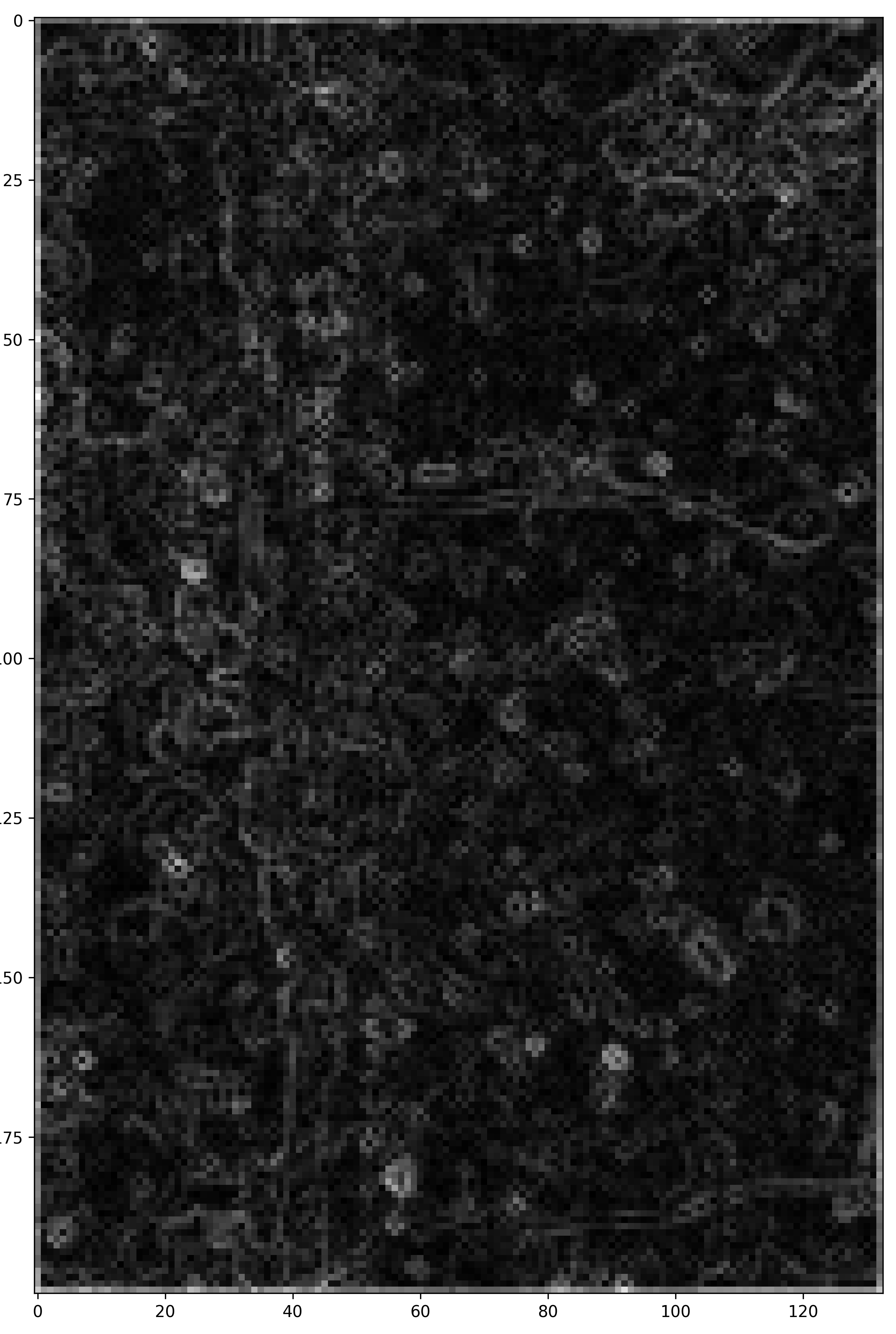
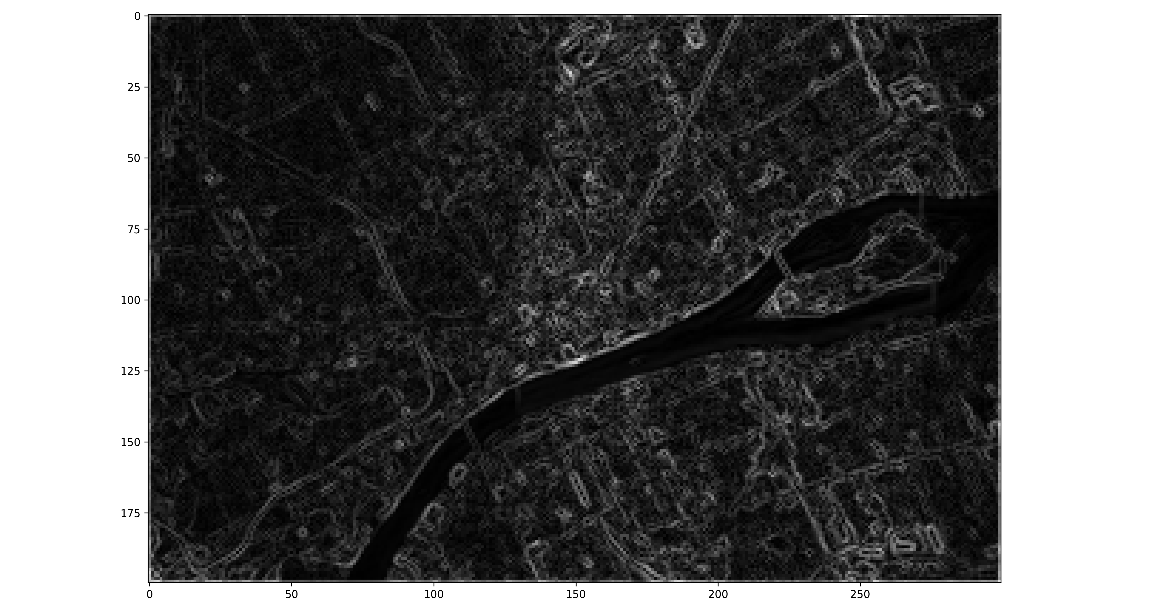
Generate image of gradient magnitudes for San Francisco image
Generate image of gradient magnitudes for Salt Lake City image
# Save gradient magnitudes of Salt Lake City in image form

# plt.figure(figsize=(8, 15))
# #plt.title('Salt Lake City, UT Gradient Magnitudes')
# plt.imshow(mag_list[1], cmap="gray")
# plt.axis("on")
# #plt.show()
# plt.tight_layout()
# plt.savefig("images/plots/aerial_cities/salt_lake_mag.png", dpi=300)
Generate image of gradient magnitudes for Detroit image
Create Data Frame for Each Image
Create Histograms of Gradient Magnitudes and Angles for Aerial Cityscapes
Plot histogram of San Francisco, CA gradient magnitudes and define the magnitude level for later filtering
# SF histogram of gradient mags
sf_histogram_mag_plot <-
ggplot(standard_df_list[[1]],
aes(x = mag)) +
geom_histogram(colour = "black", fill = "lightblue") +
scale_x_continuous() +
labs(x = "Gradient Magnitude",
y = "Count",
title = "San Francisco Cityscape Image Histogram of Gradient Magnitudes"
) +
theme_minimal() +
theme(plot.title = element_text(hjust = 0.5))
# sf mag filter level
sf_mag_filter <- 0.4
# save image
ggsave("images/plots/aerial_cities/sf_histogram_mag_plot.jpg",
sf_histogram_mag_plot,
width = 6,
height = 4,
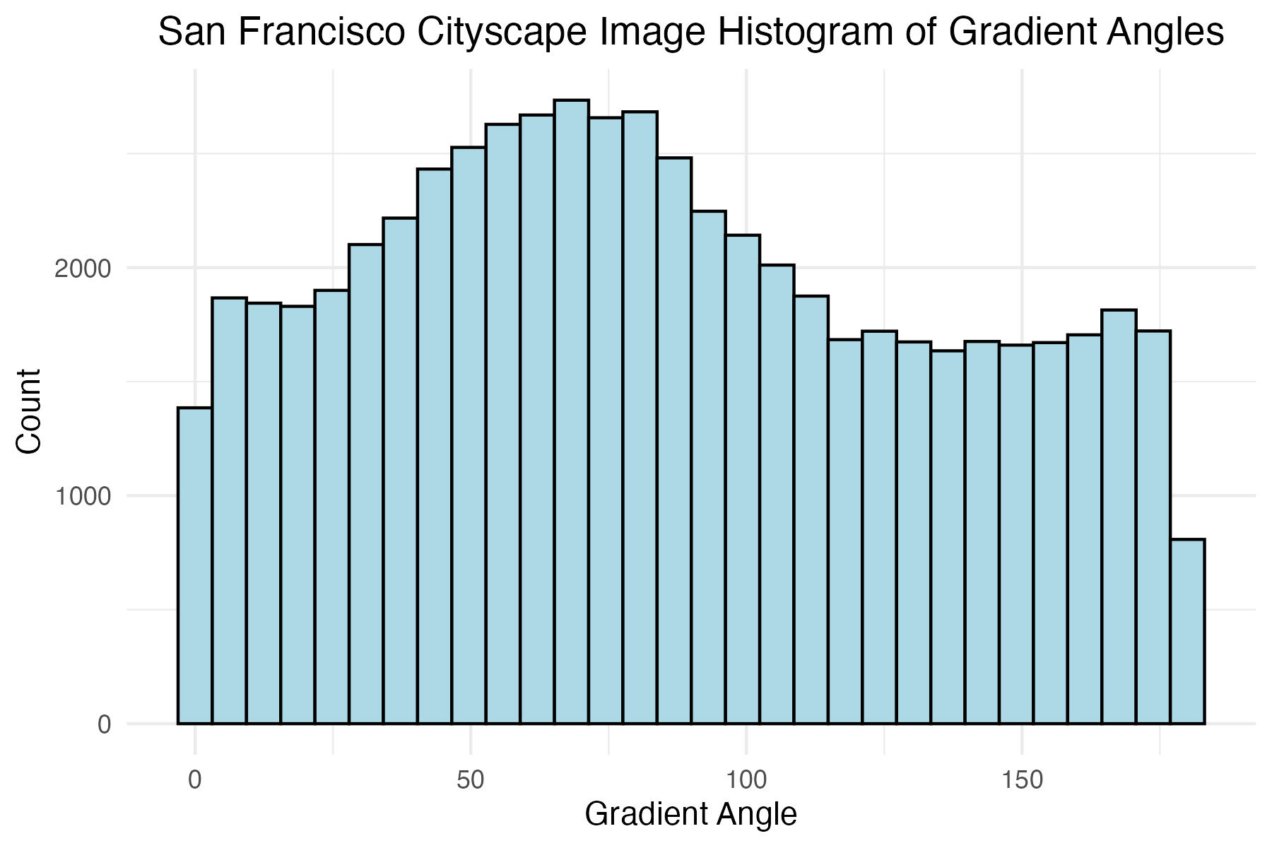
dpi = 300)Plot histogram of San Francisco, CA gradient angles
# SF histogram of gradient angles
sf_histogram_theta_plot <-
ggplot(standard_df_list[[1]],
aes(x = theta)) +
geom_histogram(colour = "black", fill = "lightblue") +
scale_x_continuous() +
labs(x = "Gradient Angle",
y = "Count",
title = "San Francisco Cityscape Image Histogram of Gradient Angles"
) +
theme_minimal() +
theme(plot.title = element_text(hjust = 0.5))
# save image
ggsave("images/plots/aerial_cities/sf_histogram_theta_plot.jpg",
sf_histogram_theta_plot,
width = 6,
height = 4,
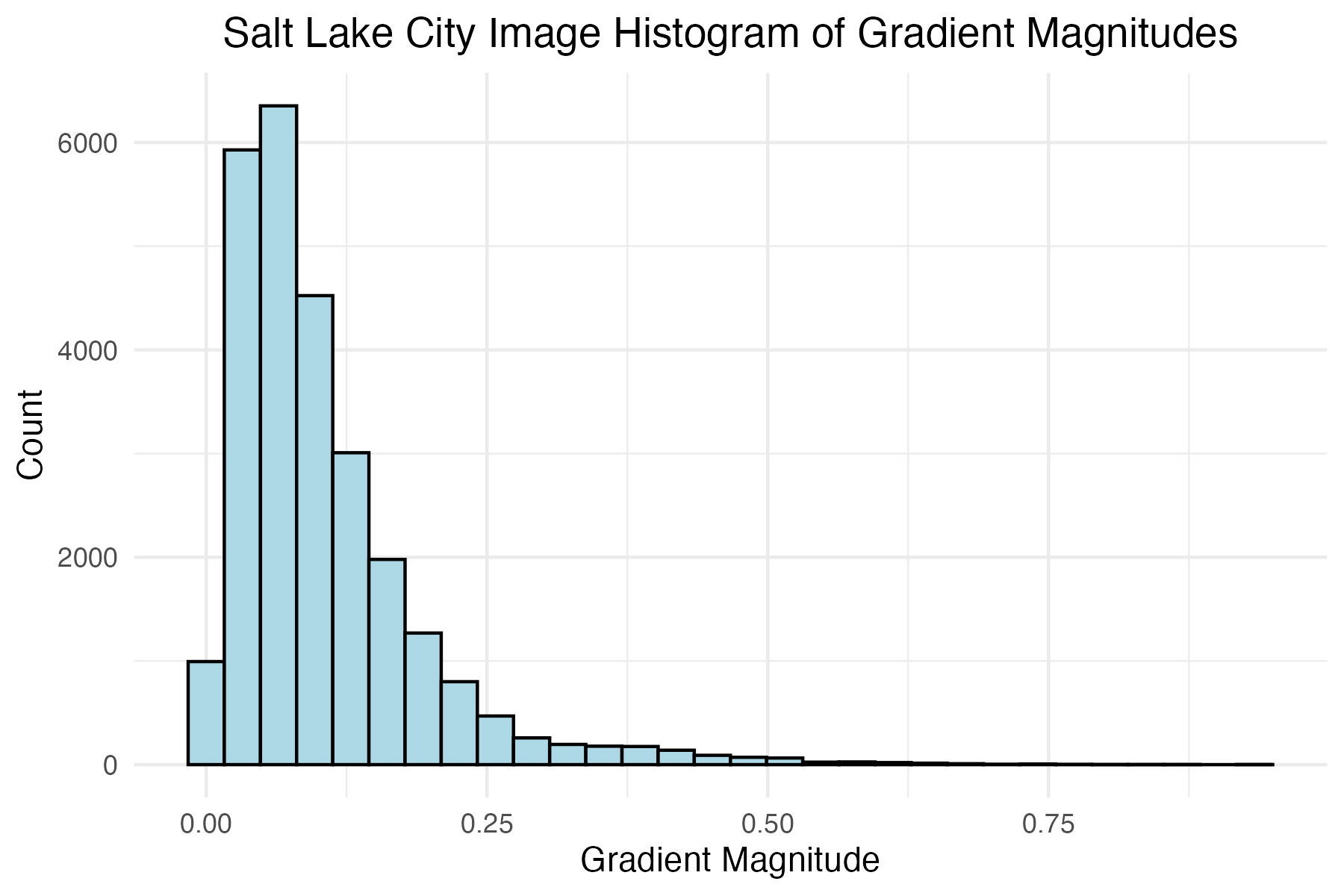
dpi = 300)Plot histogram of Salt Lake City, UT gradient magnitudes and define the magnitude level for later filtering
# slc histogram of gradient mags
salt_lake_histogram_mag_plot <-
ggplot(standard_df_list[[2]],
aes(x = mag)) +
geom_histogram(colour = "black", fill = "lightblue") +
scale_x_continuous() +
labs(x = "Gradient Magnitude",
y = "Count",
title = "Salt Lake City Image Histogram of Gradient Magnitudes"
) +
theme_minimal() +
theme(plot.title = element_text(hjust = 0.5))
# SLC mag filter level
salt_lake_mag_filter <- 0.12
# save image
ggsave("images/plots/aerial_cities/salt_lake_histogram_mag_plot.jpg",
salt_lake_histogram_mag_plot,
width = 6,
height = 4,
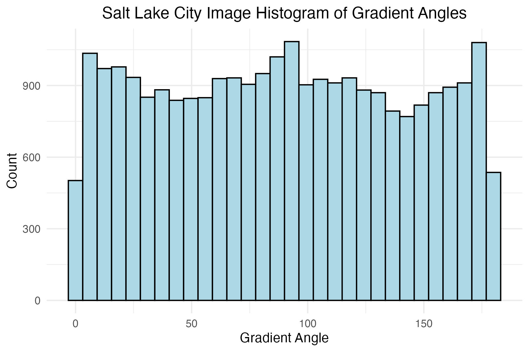
dpi = 300)Plot histogram of Salt Lake City, UT gradient angles
# slc histogram of gradient angles
salt_lake_histogram_theta_plot <-
ggplot(standard_df_list[[2]],
aes(x = theta)) +
geom_histogram(colour = "black", fill = "lightblue") +
scale_x_continuous() +
labs(x = "Gradient Angle",
y = "Count",
title = "Salt Lake City Image Histogram of Gradient Angles"
) +
theme_minimal() +
theme(plot.title = element_text(hjust = 0.5))
# save image
ggsave("images/plots/aerial_cities/salt_lake_histogram_theta_plot.jpg",
salt_lake_histogram_theta_plot,
width = 6,
height = 4,
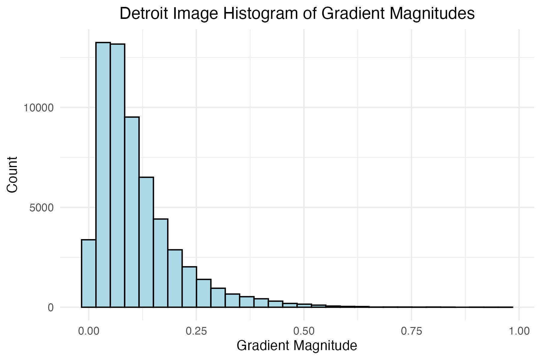
dpi = 300)Plot histogram of Detroit, MI gradient magnitudes and define the magnitude level for later filtering
# Detroit histogram of gradient mags
detroit_histogram_mag_plot <-
ggplot(standard_df_list[[3]],
aes(x = mag)) +
geom_histogram(colour = "black", fill = "lightblue") +
scale_x_continuous() +
labs(x = "Gradient Magnitude",
y = "Count",
title = "Detroit Image Histogram of Gradient Magnitudes"
) +
theme_minimal() +
theme(plot.title = element_text(hjust = 0.5))
# Detroit mag filter level
detroit_mag_filter <- 0.15
ggsave("images/plots/aerial_cities/detroit_histogram_mag_plot.jpg",
detroit_histogram_mag_plot,
width = 6,
height = 4,
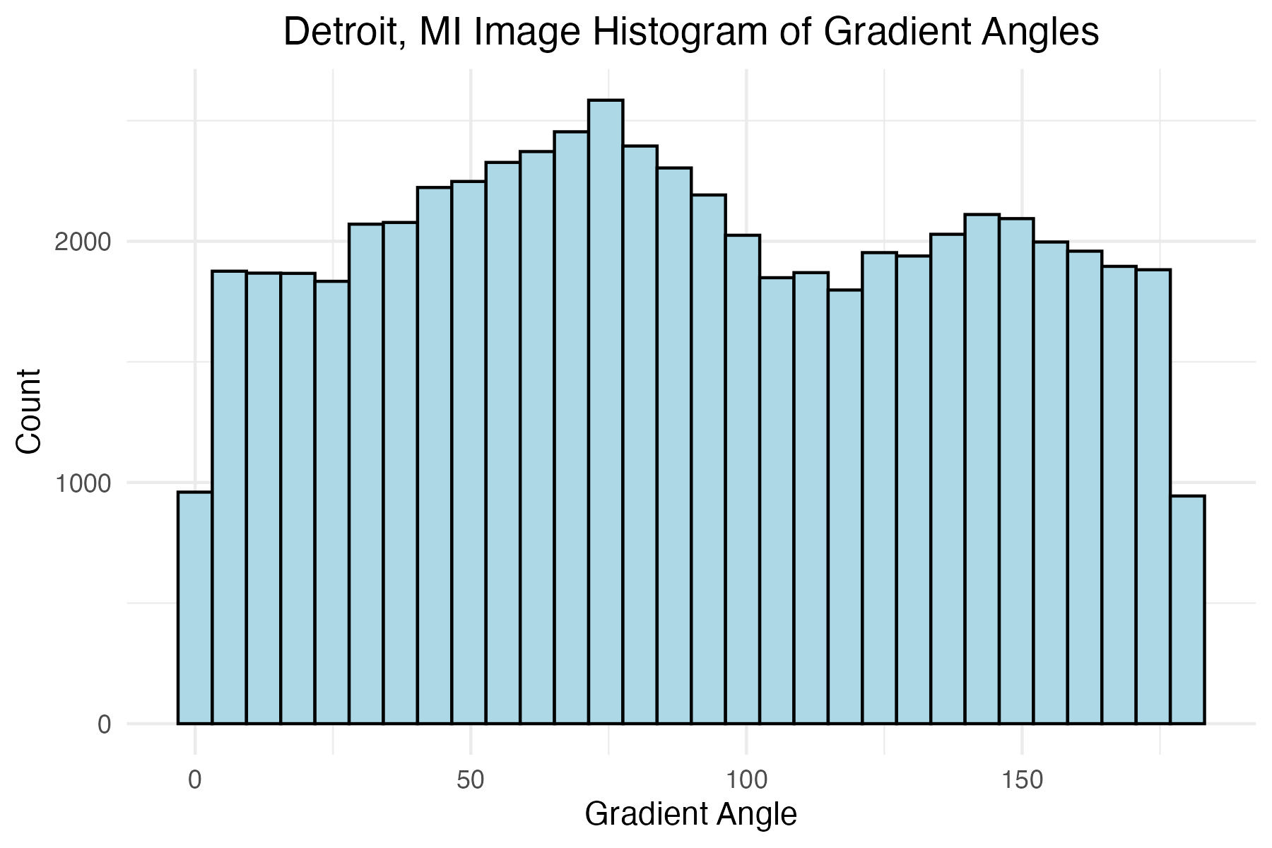
dpi = 300)Plot histogram of Detroit, MI gradient angles
# Detroit histogram of gradient angles
detroit_histogram_theta_plot <-
  ggplot(standard_df_list[[3]],
         aes(x = theta)) +
  geom_histogram(colour = "black", fill = "lightblue") +
  scale_x_continuous() +
  labs(x = "Gradient Angle",
       y = "Count",
       title = "Detroit, MI Image Histogram of Gradient Angles"
       ) +
  theme_minimal() +
  theme(plot.title = element_text(hjust = 0.5))

# save image
ggsave("images/plots/aerial_cities/detroit_histogram_theta_plot.jpg",
       detroit_histogram_theta_plot,
       width = 6,
       height = 4,
       dpi = 300)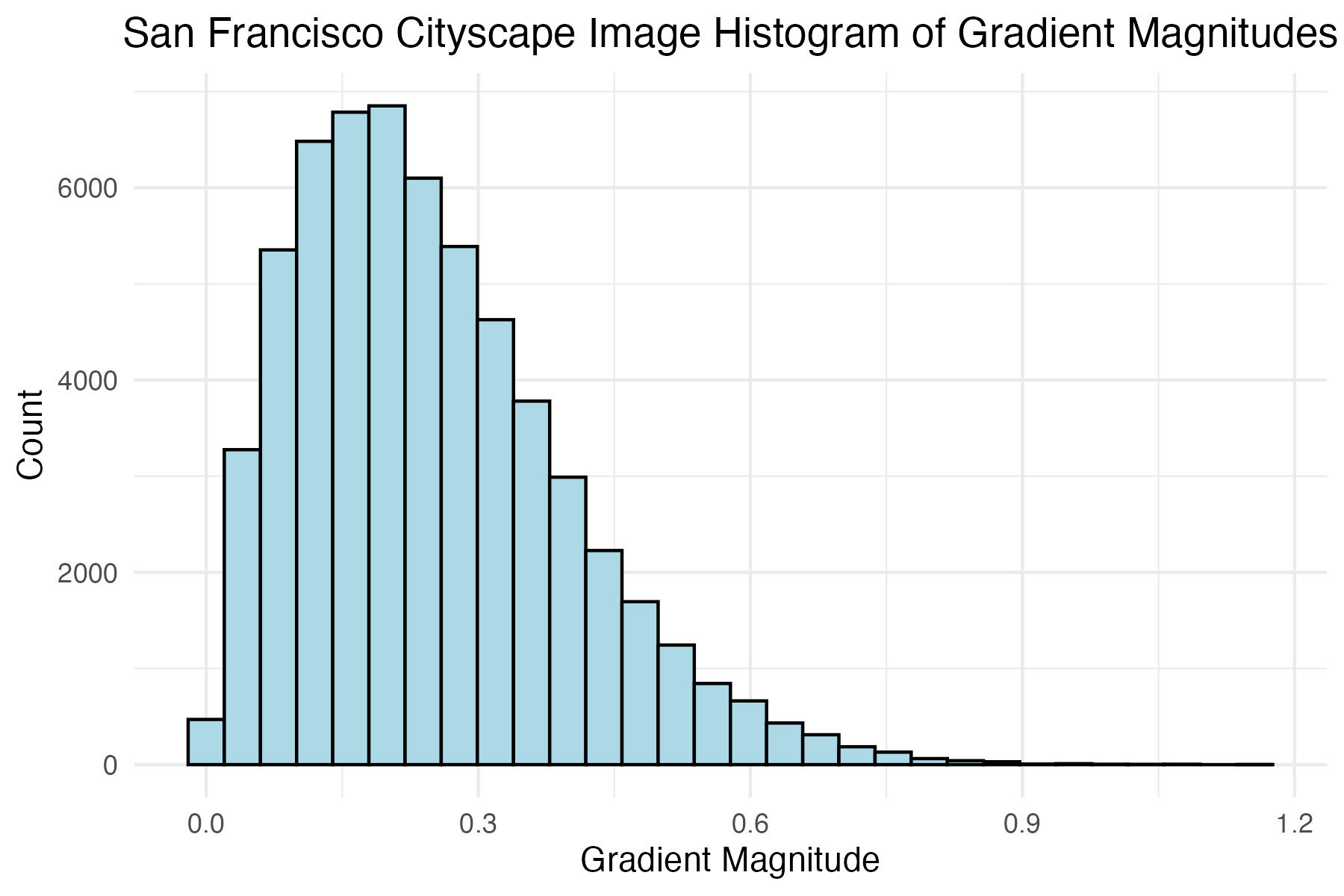
Build New Distributed Histogram Data Frames
Function for calculating values for each bin of distributed histogram
# function to calculate the contributions to neighboring bins
calculate_bin_contributions <- function(angle, magnitude, num_bins) {
  bin_width <- 180 / num_bins
  contributions <- numeric(num_bins)

  # get the central bin
  central_bin <- floor(angle / bin_width) %% num_bins
  next_bin <- (central_bin + 1) %% num_bins

  # get contributions to neighboring bins
  weight <- (1 - abs((angle %% bin_width) / bin_width)) * magnitude

  contributions[central_bin + 1] <- weight
  contributions[next_bin + 1] <- magnitude - weight

  return(list(contributions[1],
         contributions[2],
         contributions[3],
         contributions[4],
         contributions[5],
         contributions[6],
         contributions[7],
         contributions[8],
         contributions[9])
         )
}
Filter each data set of aerial image gradients and angles to only contain observations with magnitudes greater than or equal to the respective magnitude levels determined above
# Create filtered data frames using the filter levels
# for magnitudes defined above, store all in a list
filtered_aerial_standard_df_list <-list(sf_hog_df %>%
                                   filter(mag >= sf_mag_filter),
                                 salt_lake_hog_df %>%
                                   filter(mag >= salt_lake_mag_filter),
                                 detroit_hog_df %>%
                                   filter(mag >= detroit_mag_filter))
For each image calculate the contribution to each bin for the disttribued histogram
# empty list for storing new distributed histogram data frames
aerial_contribution_df_list <- list()

# Define the number of bins
num_bins <- 9

# iterate through each filtered standard data frame
for (i in 1:length(filtered_aerial_standard_df_list)){

  aerial_contribution_hog_df <-
    filtered_aerial_standard_df_list[[i]] %>%
    rowwise() %>%
    mutate(`0` = calculate_bin_contributions(theta, mag, 9)[[1]],
           `20` = calculate_bin_contributions(theta, mag, 9)[[2]],
           `40` = calculate_bin_contributions(theta, mag, 9)[[3]],
           `60` = calculate_bin_contributions(theta, mag, 9)[[4]],
           `80` = calculate_bin_contributions(theta, mag, 9)[[5]],
           `100` = calculate_bin_contributions(theta, mag, 9)[[6]],
           `120` = calculate_bin_contributions(theta, mag, 9)[[7]],
           `140` = calculate_bin_contributions(theta, mag, 9)[[8]],
           `160` = calculate_bin_contributions(theta, mag, 9)[[9]],
           )

  # rearrange into same tidy format
  aerial_split_histo_df <-
    aerial_contribution_hog_df %>%
    pivot_longer(names_to = "bin",
                 values_to = "contribution",
                 cols = 4:ncol(aerial_contribution_hog_df)) %>%
    mutate(bin = as.numeric(bin)) %>%
    group_by(bin) %>%
    summarise(contribution_sum = sum(contribution))

  # add to list for storage
  aerial_contribution_df_list[[i]] <- aerial_split_histo_df

}
Generate Polar Plots for Images Using Standard Histogram Binning Technique
Polar plot of San Francisco, CA histogram of gradient angles using standard binning technique
# SF polar plot
sf_plot <-
ggplot(filtered_aerial_standard_df_list[[1]],
aes(x = theta)) +
geom_histogram(colour = "black",
fill = "lightblue",
breaks = seq(0, 360, length.out = 17.5),
bins = 9) +
coord_polar(
theta = "x",
start = 0,
direction = 1) +
scale_x_continuous(limits = c(0,360),
breaks = c(0, 45, 90, 135, 180, 225, 270, 315),
labels = c("N", "NE", "E", "SE", "S", "SW", "W", "NW")
)+
labs(title = "Polar Plot of San Francisco, CA Image
Using Standard HOG Technique") +
theme_minimal() +
labs(x = "") +
theme(axis.title.y = element_blank(),
plot.title = element_text(hjust = 0.5))
# save image
ggsave("images/plots/aerial_cities/sf_standard_polar_plot.jpg",
sf_plot,
width = 6,
height = 4,
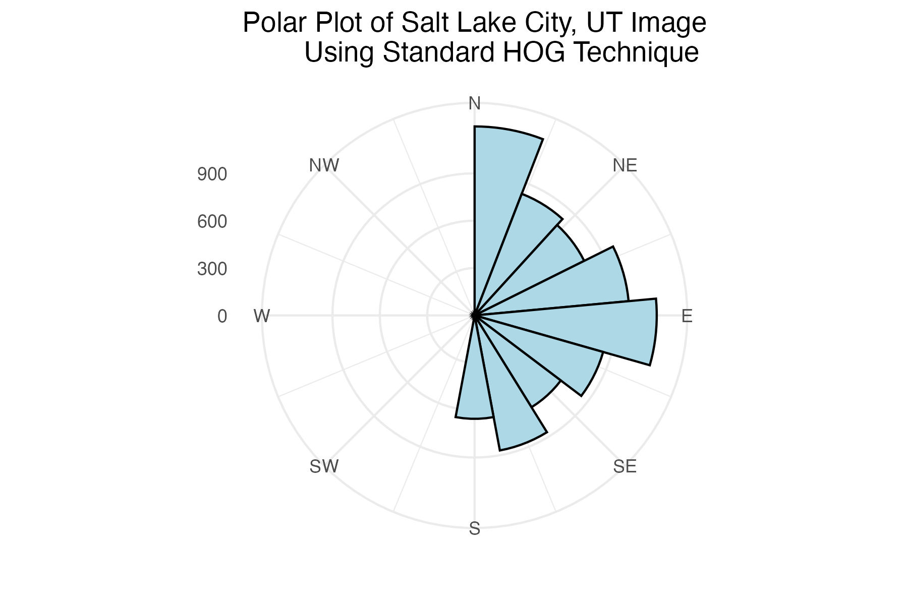
dpi = 300)Polar plot of Salt Lake City, UT histogram of gradient angles using standard binning technique
# SLC plot
salt_lake_plot <-
ggplot(filtered_aerial_standard_df_list[[2]],
aes(x = theta)) +
geom_histogram(colour = "black",
fill = "lightblue",
breaks = seq(0, 360, length.out = 17.5),
bins = 9) +
coord_polar(
theta = "x",
start = 0,
direction = 1) +
scale_x_continuous(limits = c(0,360),
breaks = c(0, 45, 90, 135, 180, 225, 270, 315),
labels = c("N", "NE", "E", "SE", "S", "SW", "W", "NW")
)+
labs(title = "Polar Plot of Salt Lake City, UT Image
Using Standard HOG Technique") +
theme_minimal() +
labs(x = "") +
theme(axis.title.y = element_blank(),
plot.title = element_text(hjust = 0.5))
# save image
ggsave("images/plots/aerial_cities/salt_lake_standard_polar_plot.jpg",
salt_lake_plot,
width = 6,
height = 4,
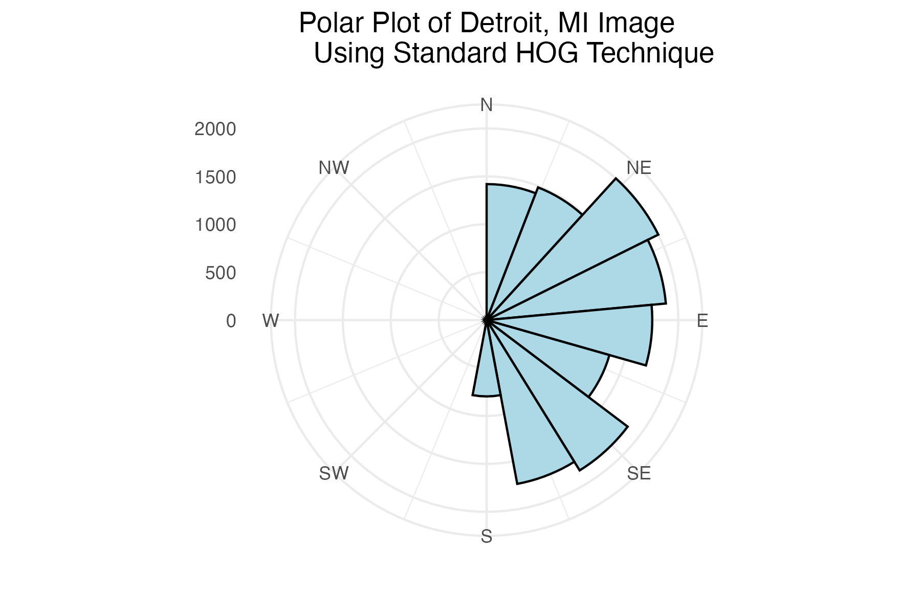
dpi = 300)Polar plot of Detroit, MI histogram of gradient angles using standard binning technique
# Detroit plot
detroit_plot <-
  ggplot(filtered_aerial_standard_df_list[[3]],
         aes(x = theta)) +
  geom_histogram(colour = "black",
                 fill = "lightblue",
                 breaks = seq(0, 360, length.out = 17.5),
                 bins = 9) +
  coord_polar(
    theta = "x",
    start = 0,
    direction = 1) +
  scale_x_continuous(limits = c(0,360),
    breaks = c(0, 45, 90, 135, 180, 225, 270, 315),
    labels = c("N", "NE", "E", "SE", "S", "SW", "W", "NW")
  )+
  labs(title = "Polar Plot of Detroit, MI Image
       Using Standard HOG Technique") +
  theme_minimal() +
  labs(x = "") +
  theme(axis.title.y = element_blank(),
        plot.title = element_text(hjust = 0.5))

# save image
ggsave("images/plots/aerial_cities/detroit_standard_polar_plot.jpg",
       detroit_plot,
       width = 6,
       height = 4,
       dpi = 300)
Generate Polar Plots for Images Using Distributed Histogram Binning Technique
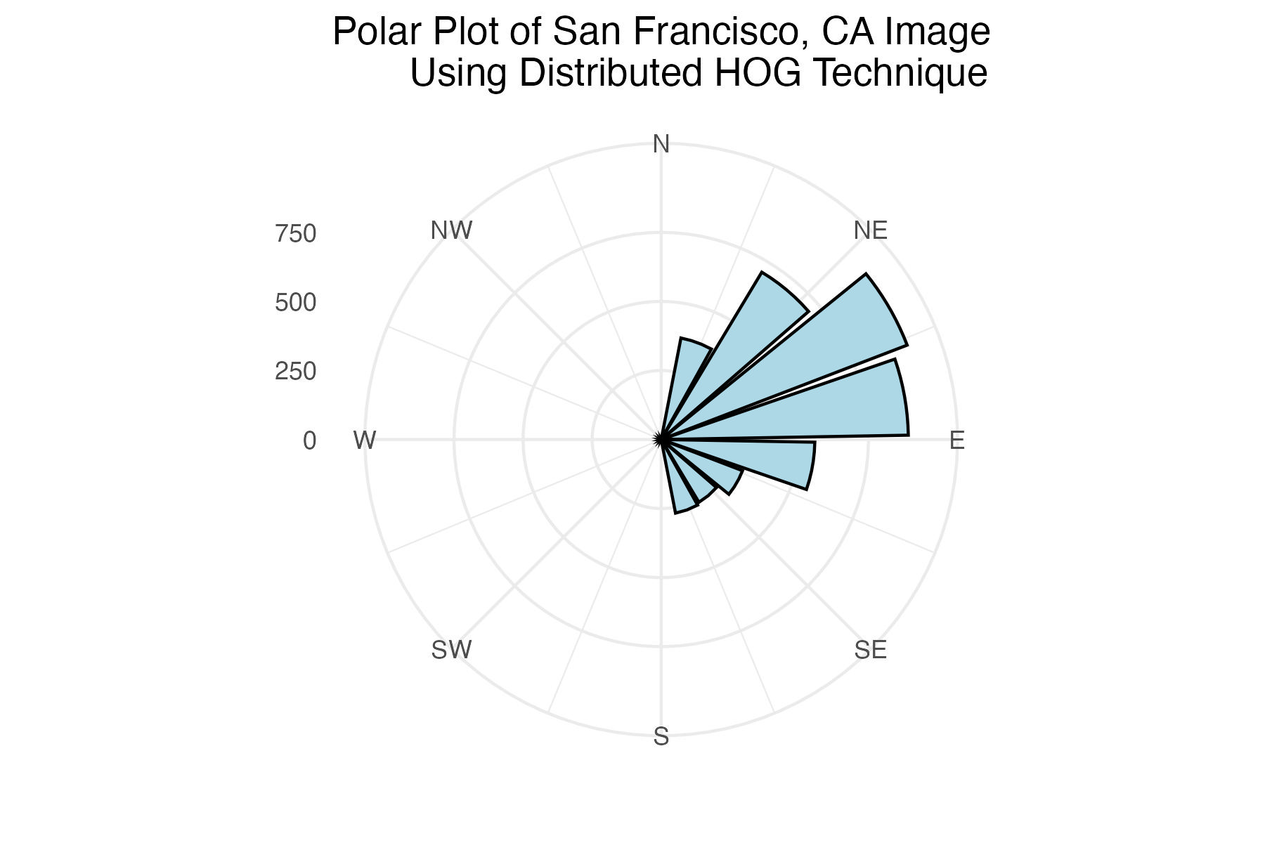
Polar plot of San Francisco, CA histogram of gradient angles using distributed binning technique
# SF plot
sf_split_plot <-
ggplot(aerial_contribution_df_list[[1]],
aes(x = bin, y = contribution_sum)) +
geom_histogram(stat = "identity",
colour = "black",
fill = "lightblue",
breaks = seq(0, 360, length.out = 17.5),
bins = 9) +
coord_polar(
theta = "x",
start = 0,
direction = 1) +
scale_x_continuous(limits = c(0,360),
breaks = c(0, 45, 90, 135, 180, 225, 270, 315),
labels = c("N", "NE", "E", "SE", "S", "SW", "W", "NW")
)+
labs(title = "Polar Plot of San Francisco, CA Image
Using Distributed HOG Technique") +
theme_minimal() +
labs(x = "") +
theme(axis.title.y = element_blank(),
plot.title = element_text(hjust = 0.5))
# save image
ggsave("images/plots/aerial_cities/sf_contribution_polar_plot.jpg",
sf_split_plot,
width = 6,
height = 4,
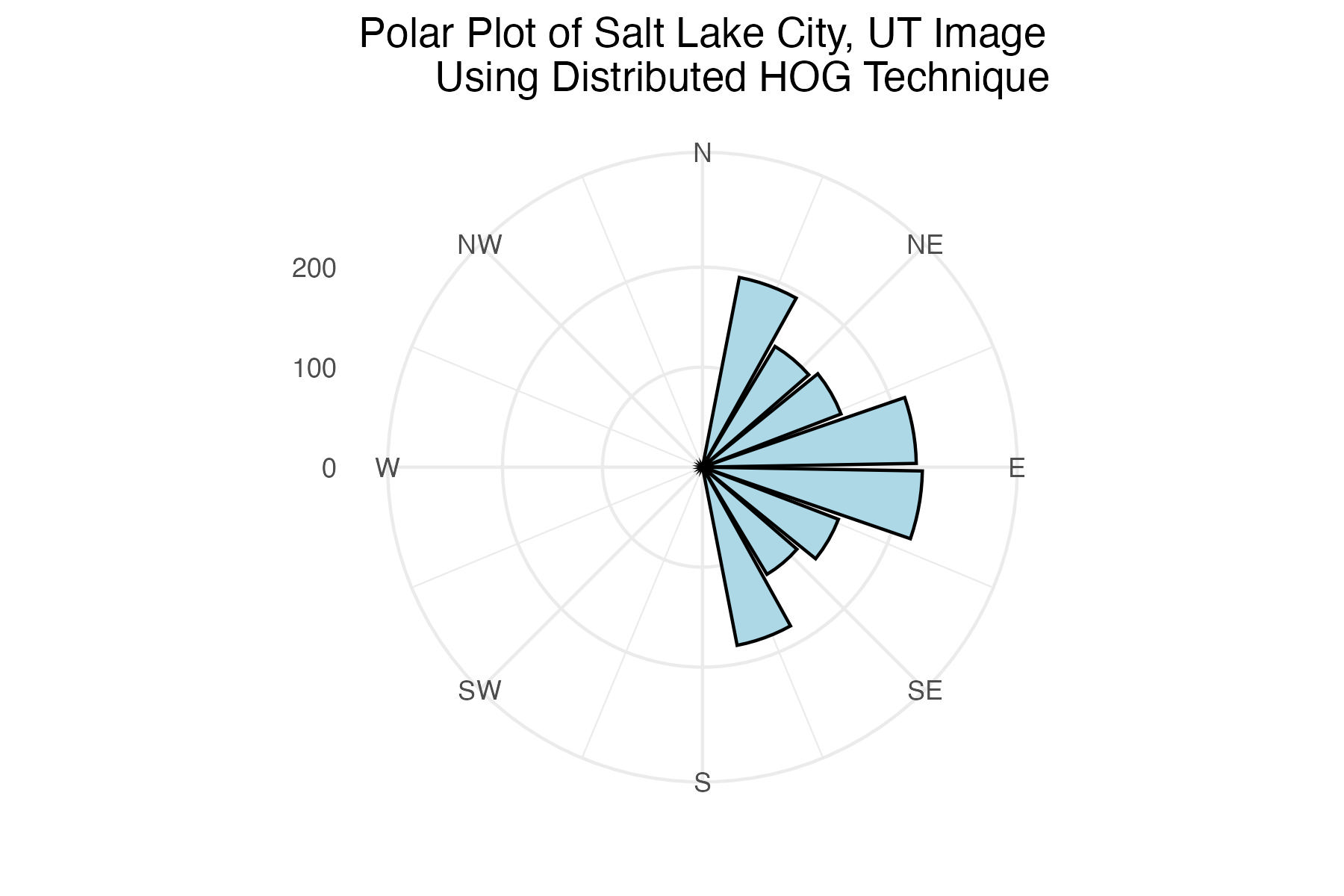
dpi = 300)Polar plot of Salt Lake City, UT histogram of gradient angles using distributed binning technique
# SLC plot
salt_lake_split_plot <-
ggplot(aerial_contribution_df_list[[2]],
aes(x = bin, y = contribution_sum)) +
geom_histogram(stat = "identity",
colour = "black",
fill = "lightblue",
breaks = seq(0, 360, length.out = 17.5),
bins = 9) +
coord_polar(
theta = "x",
start = 0,
direction = 1) +
scale_x_continuous(limits = c(0,360),
breaks = c(0, 45, 90, 135, 180, 225, 270, 315),
labels = c("N", "NE", "E", "SE", "S", "SW", "W", "NW")
)+
labs(title = "Polar Plot of Salt Lake City, UT Image
Using Distributed HOG Technique") +
theme_minimal() +
labs(x = "") +
theme(axis.title.y = element_blank(),
plot.title = element_text(hjust = 0.5))
# save image
ggsave("images/plots/aerial_cities/salt_lake_contribution_polar_plot.jpg",
salt_lake_split_plot,
width = 6,
height = 4,
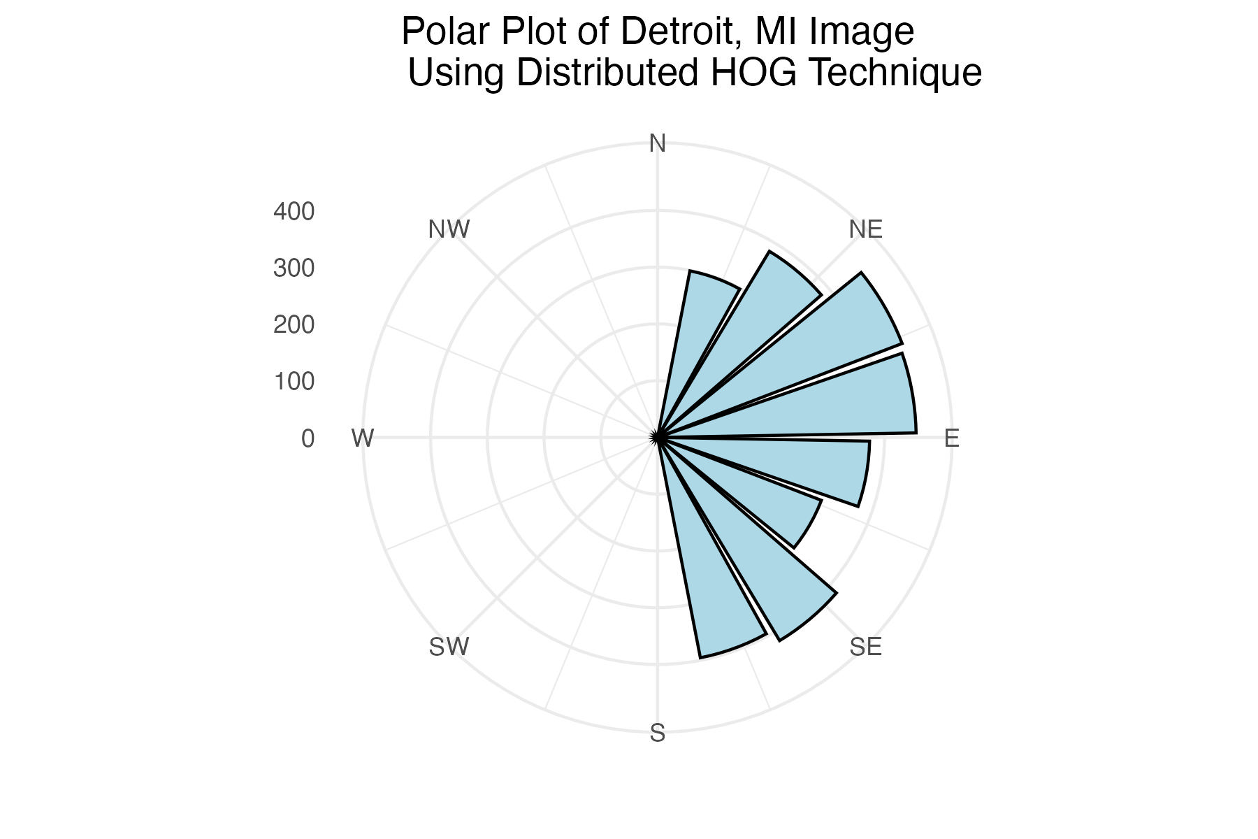
dpi = 300)Polar plot of Detroit, MI histogram of gradient angles using distributed binning technique
# Detroit plot
detroit_split_plot <-
  ggplot(aerial_contribution_df_list[[3]],
         aes(x = bin, y = contribution_sum)) +
  geom_histogram(stat = "identity",
                 colour = "black",
                 fill = "lightblue",
                 breaks = seq(0, 360, length.out = 17.5),
                 bins = 9) +
  coord_polar(
    theta = "x",
    start = 0,
    direction = 1) +
  scale_x_continuous(limits = c(0,360),
    breaks = c(0, 45, 90, 135, 180, 225, 270, 315),
    labels = c("N", "NE", "E", "SE", "S", "SW", "W", "NW")
  )+
  labs(title = "Polar Plot of Detroit, MI Image
       Using Distributed HOG Technique") +
  theme_minimal() +
  labs(x = "") +
  theme(axis.title.y = element_blank(),
        plot.title = element_text(hjust = 0.5))

# save image
ggsave("images/plots/aerial_cities/detroit_contribution_polar_plot.jpg",
       detroit_split_plot,
       width = 6,
       height = 4,
       dpi = 300)
Save an arranged image of the 3 distributed-binned polar plots side-by-side
Discussion
The San Francisco image delivered the most promising results due to its closer zoom level compared to the Salt Lake City and Detroit images. Angles in the seventy-degree range emerged as the most frequent, accurately reflecting the slightly diagonal west-east streets of downtown San Francisco. The layout of Salt Lake City significantly influenced the results of its polar plot. With its narrow vertical grid layout, the city exhibited a higher frequency of vertical angles and a smaller yet significant occurrence of horizontal gradient angles. For the images of San Francisco and Detroit, the outcomes between the Standard and Distributed binning techniques exhibited similar results. However, for Salt Lake City, the Distributed technique notably favored a higher frequency of both vertical and horizontal angles.