5 Grass Images
Motivation
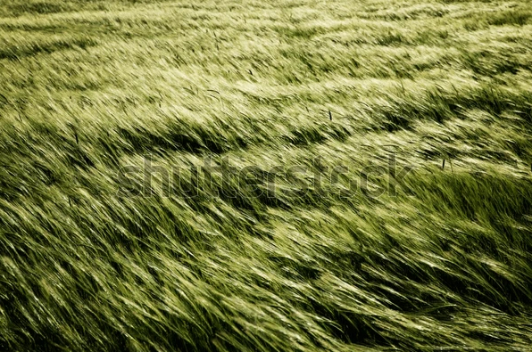
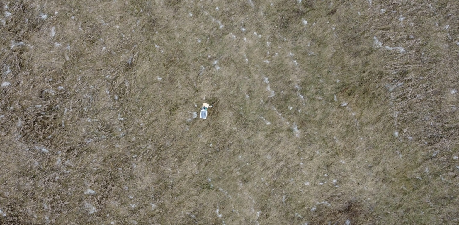
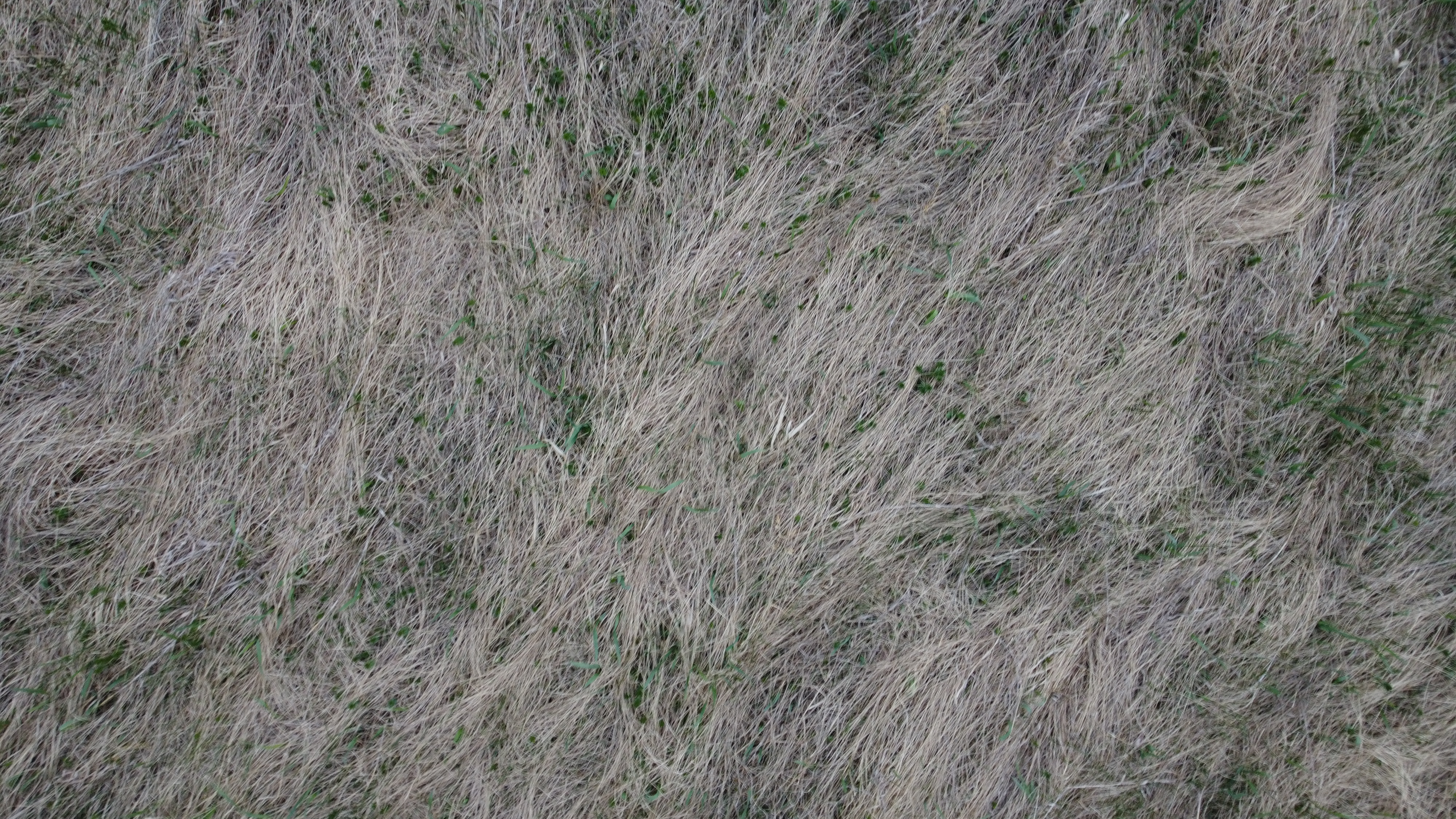
Use images from the internet and St. Lawrence University’s Living Laboratory to determine if the HOG algorithm can identify dominant angles of grass lay.
Input Images
Load R Packages and Python Libraries
Code
# Load Python Libraries
import matplotlib.pyplot as plt
import pandas as pd
from skimage.io import imread, imshow
from skimage.transform import resize
from skimage.feature import hog
from skimage import data, exposure
import matplotlib.pyplot as plt
from skimage import io
from skimage import color
from skimage.transform import resize
import math
from skimage.feature import hog
import numpy as np
Collect HOG Features for Grass Images
Code
# List for storing images
img_list = []
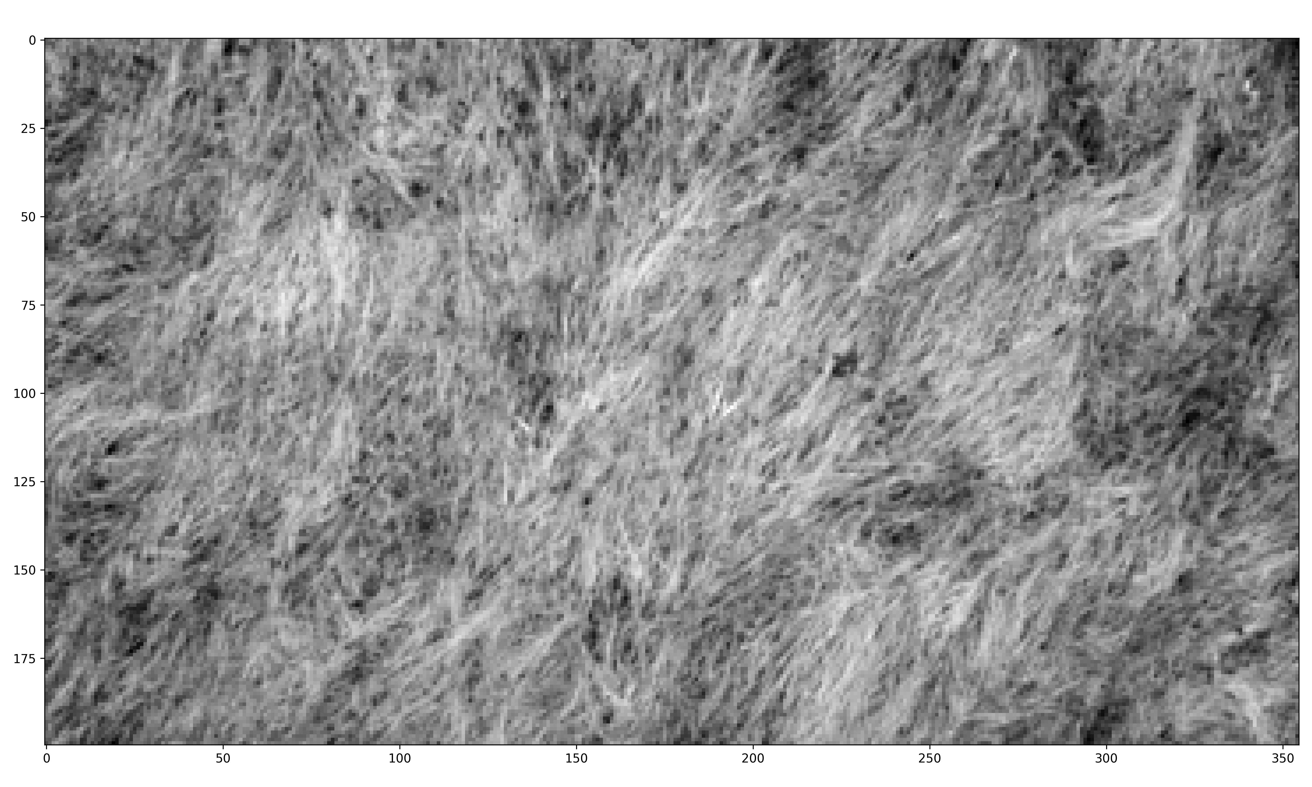
# Internet Grass Image
img_list.append(color.rgb2gray(io.imread("images/grass_image2.jpg")))
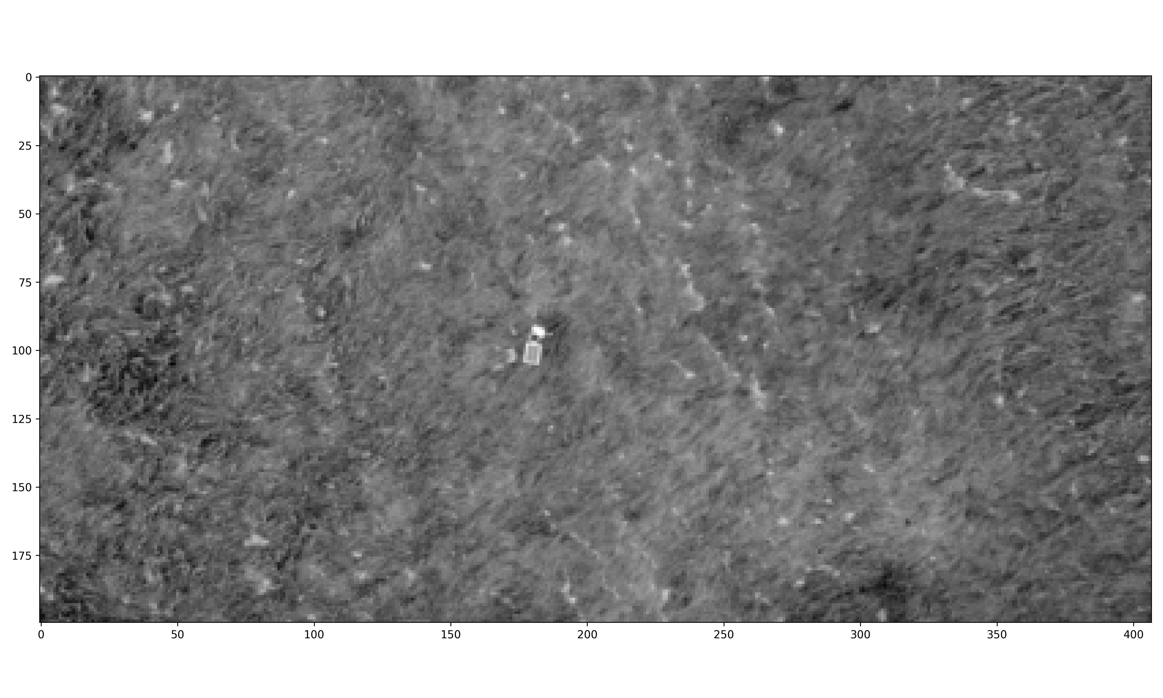
# Living Lab Rotated Aerial Grass
img_list.append(
color.rgb2gray(
io.imread("images/living_lab_aerial/aerial_grass_living_lab_rotated.jpg")))
# Living Lab Grass Close-up
img_list.append(
color.rgb2gray(
io.imread("images/living_lab_aerial/LL_zoomed_in_12.jpg")
)
)
# List to store magnitudes for each image
mag_list = []
# List to store angles for each image
theta_list = []
for x in range(len(img_list)):
# Get image of interest
img = img_list[x]
rescaled_file_path = f"images/plots/grass/{x}.jpg"
# Determine aspect Ratio
aspect_ratio = img.shape[0] / img.shape[1]
print("Aspect Ratio:", aspect_ratio)
# Hard-Code height to 200 pixels
height = 200
# Calculate witdth to maintain same aspect ratio
width = int(height / aspect_ratio)
print("Resized Width:", width)
# Resize the image
resized_img = resize(img, (height, width))
# Replace the original image with the resized image
img_list[x] = resized_img
# plt.figure(figsize=(plot_width, plot_height))
# plt.imshow(resized_img, cmap="gray")
# plt.axis("on")
# plt.tight_layout()
# plt.savefig(rescaled_file_path, dpi=300)
# plt.show()
# list for storing all magnitudes for image[x]
mag = []
# list for storing all angles for image[x]
theta = []
for i in range(height):
magnitudeArray = []
angleArray = []
for j in range(width):
if j - 1 < 0 or j + 1 >= width:
if j - 1 < 0:
Gx = resized_img[i][j + 1] - 0
elif j + 1 >= width:
Gx = 0 - resized_img[i][j - 1]
else:
Gx = resized_img[i][j + 1] - resized_img[i][j - 1]
if i - 1 < 0 or i + 1 >= height:
if i - 1 < 0:
Gy = 0 - resized_img[i + 1][j]
elif i + 1 >= height:
Gy = resized_img[i - 1][j] - 0
else:
Gy = resized_img[i + 1][j] - resized_img[i - 1][j]
magnitude = math.sqrt(pow(Gx, 2) + pow(Gy, 2))
magnitudeArray.append(round(magnitude, 9))
if Gx == 0:
angle = math.degrees(0.0)
else:
angle = math.degrees(math.atan(Gy / Gx))
if angle < 0:
angle += 180
angleArray.append(round(angle, 9))
mag.append(magnitudeArray)
theta.append(angleArray)
# add list of magnitudes to list[x]
mag_list.append(mag)
# add list of angles to angle list[x]
theta_list.append(theta)Aspect Ratio: 0.662751677852349
Resized Width: 301
Aspect Ratio: 0.4904214559386973
Resized Width: 407
Aspect Ratio: 0.5625
Resized Width: 355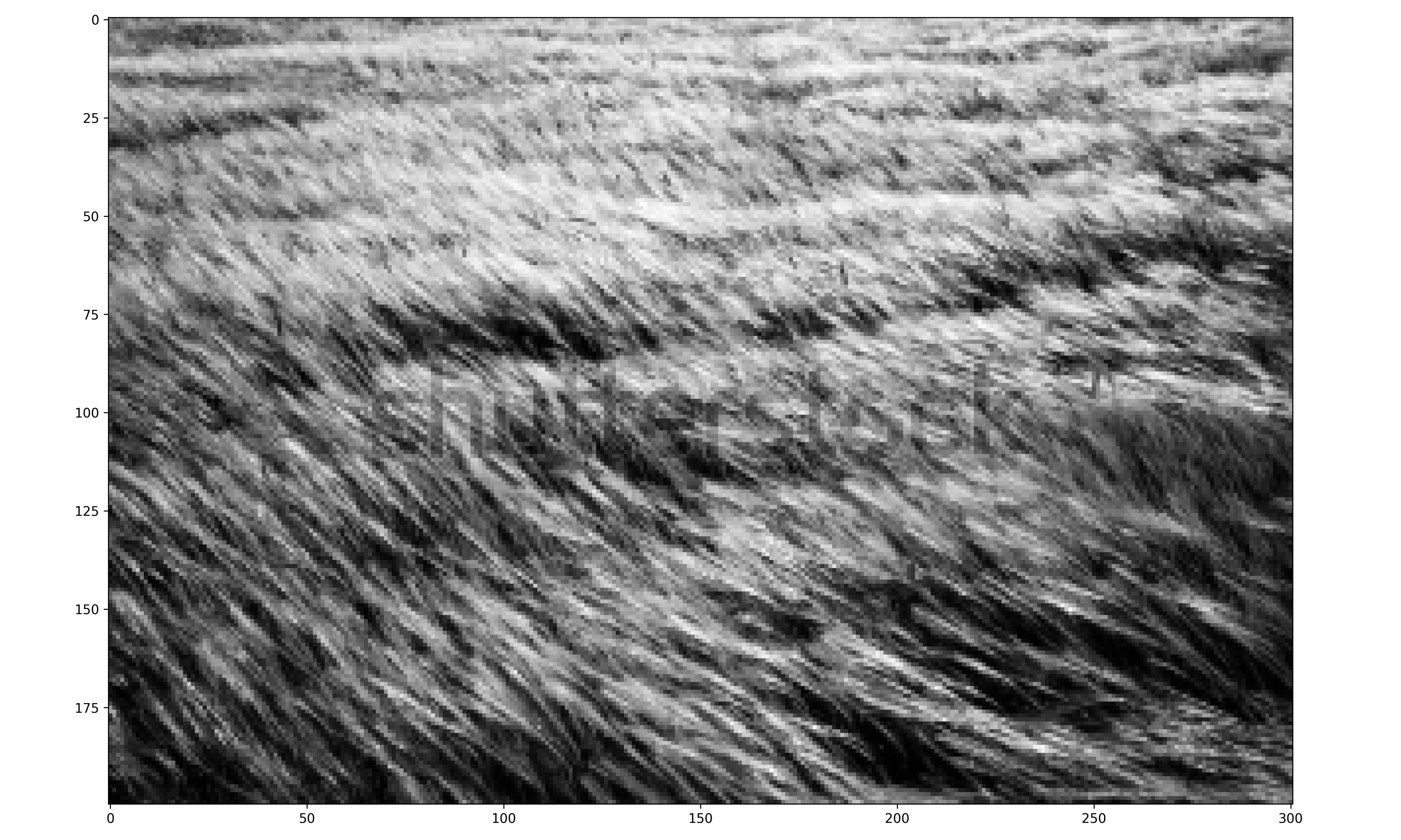
Extract Gradient Magnitudes and Angles from each Grass Image
Code
# Internet grass DF of gradient magnitudes and angles
mag_internet_grass = np.array(mag_list[0])
theta_internet_grass = np.array(theta_list[0])
# Aerial Living Lab DF of gradient magnitudes and angles
mag_aerial_living_lab = np.array(mag_list[1])
theta_aerial_living_lab = np.array(theta_list[1])
# Close-up Living Lab DF of gradient magnitudes and angles
mag_close_up_living_lab = np.array(mag_list[2])
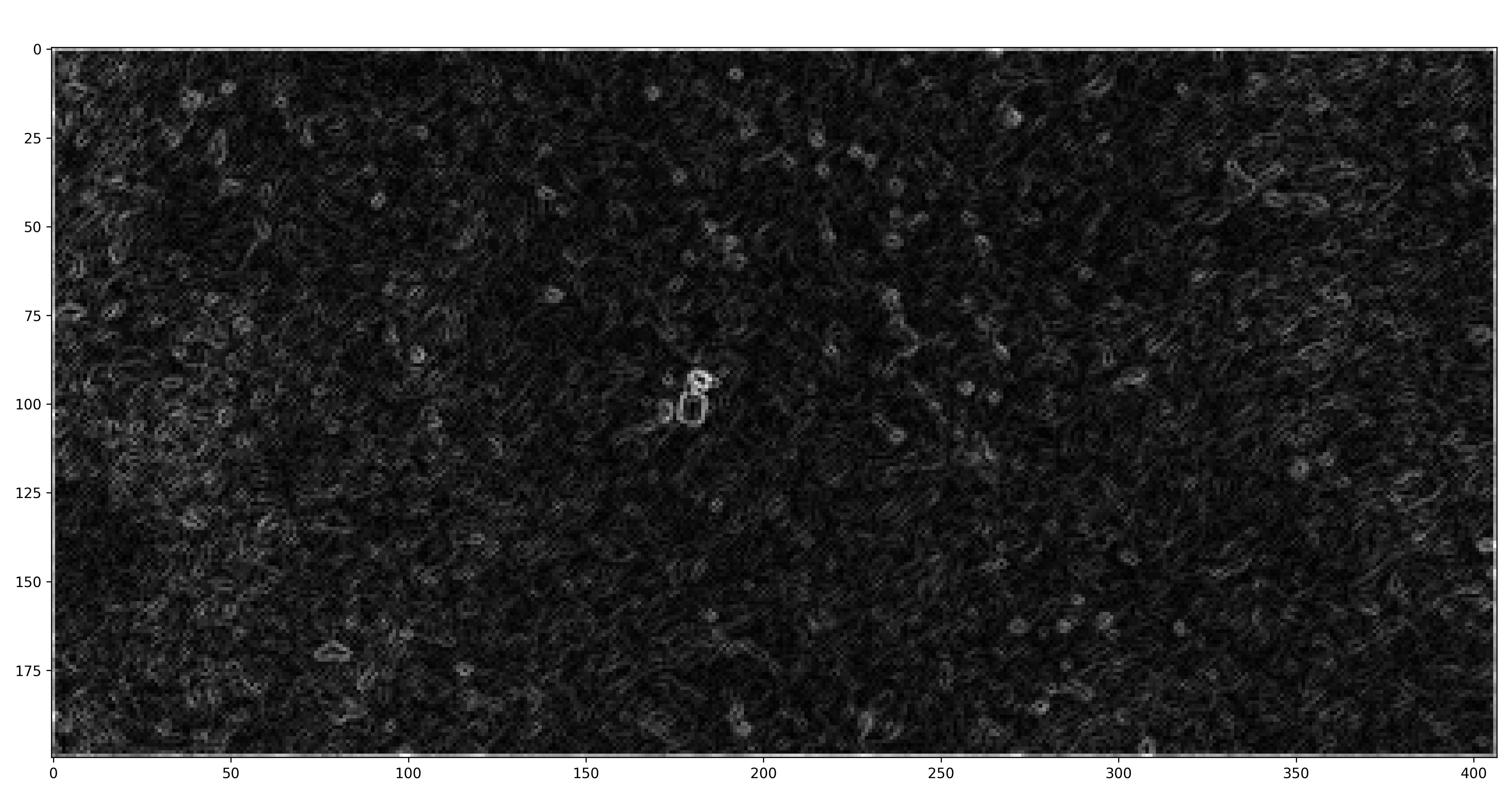
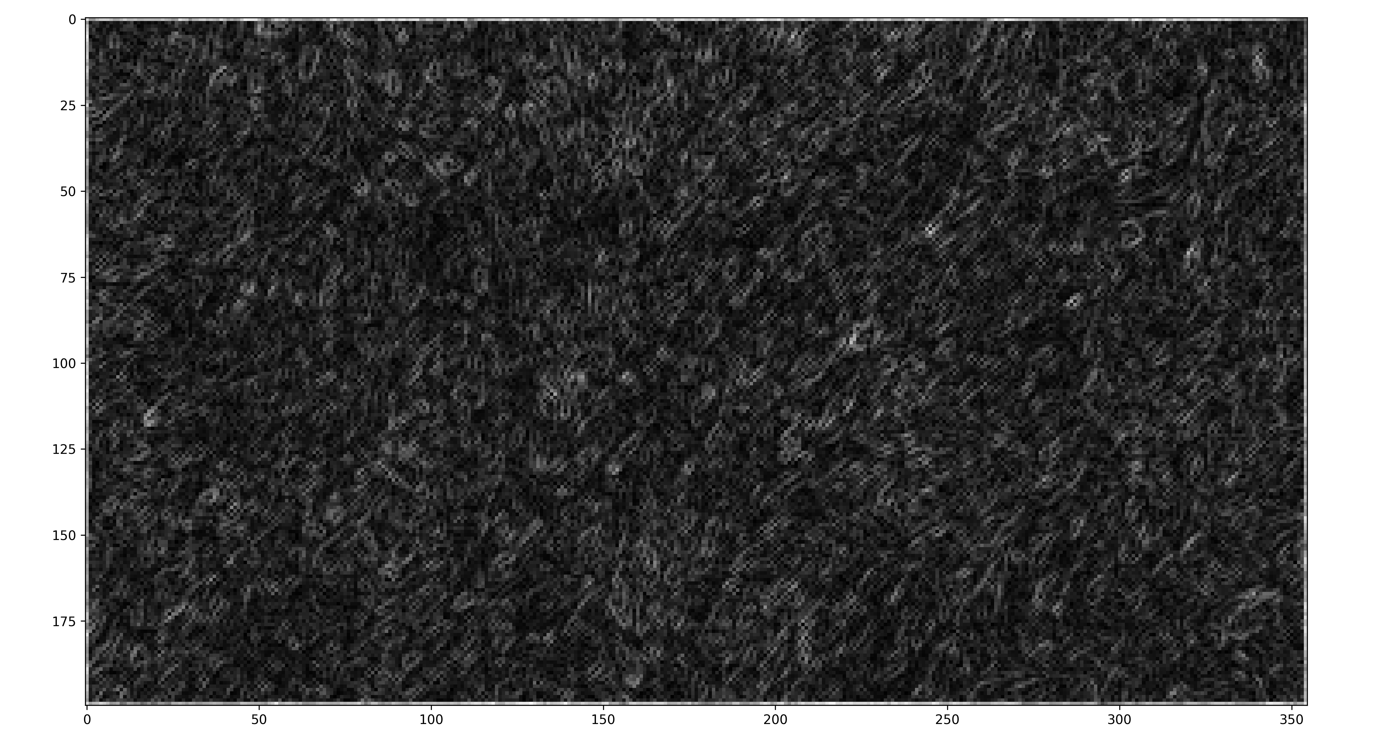
theta_close_up_living_lab = np.array(theta_list[2])Plot Gradient Magnitudes as Image for each Grass Image
Code
# Save gradient magnitudes of Internet Grass in image form

# plt.figure(figsize=(15, 8))
# #plt.title('San Francisco, CA Gradient Magnitudes')
# plt.imshow(mag_list[0], cmap="gray")
# plt.axis("on")
# #plt.show()
# plt.tight_layout()
# plt.savefig("images/plots/grass/internet_grass_mag.png", dpi=300)
Code
# Save gradient magnitudes of Aerial Living Lab in image form

# plt.figure(figsize=(15, 8))
# #plt.title('Salt Lake City, UT Gradient Magnitudes')
# plt.imshow(mag_list[1], cmap="gray")
# plt.axis("on")
# #plt.show()
# plt.tight_layout()
# plt.savefig("images/plots/grass/aerial_living_lab_grass_mag.png", dpi=300)
Code
# Save gradient magnitudes of Close-Up Living Lab in image form

# plt.figure(figsize=(15, 8))
# #plt.title('Detroit, MI Gradient Magnitudes')
# plt.imshow(mag_list[2], cmap="gray")
# plt.axis("on")
# #plt.show()
# plt.tight_layout()
# plt.savefig("images/plots/grass/close_up_living_lab_grass_mag.png", dpi=300)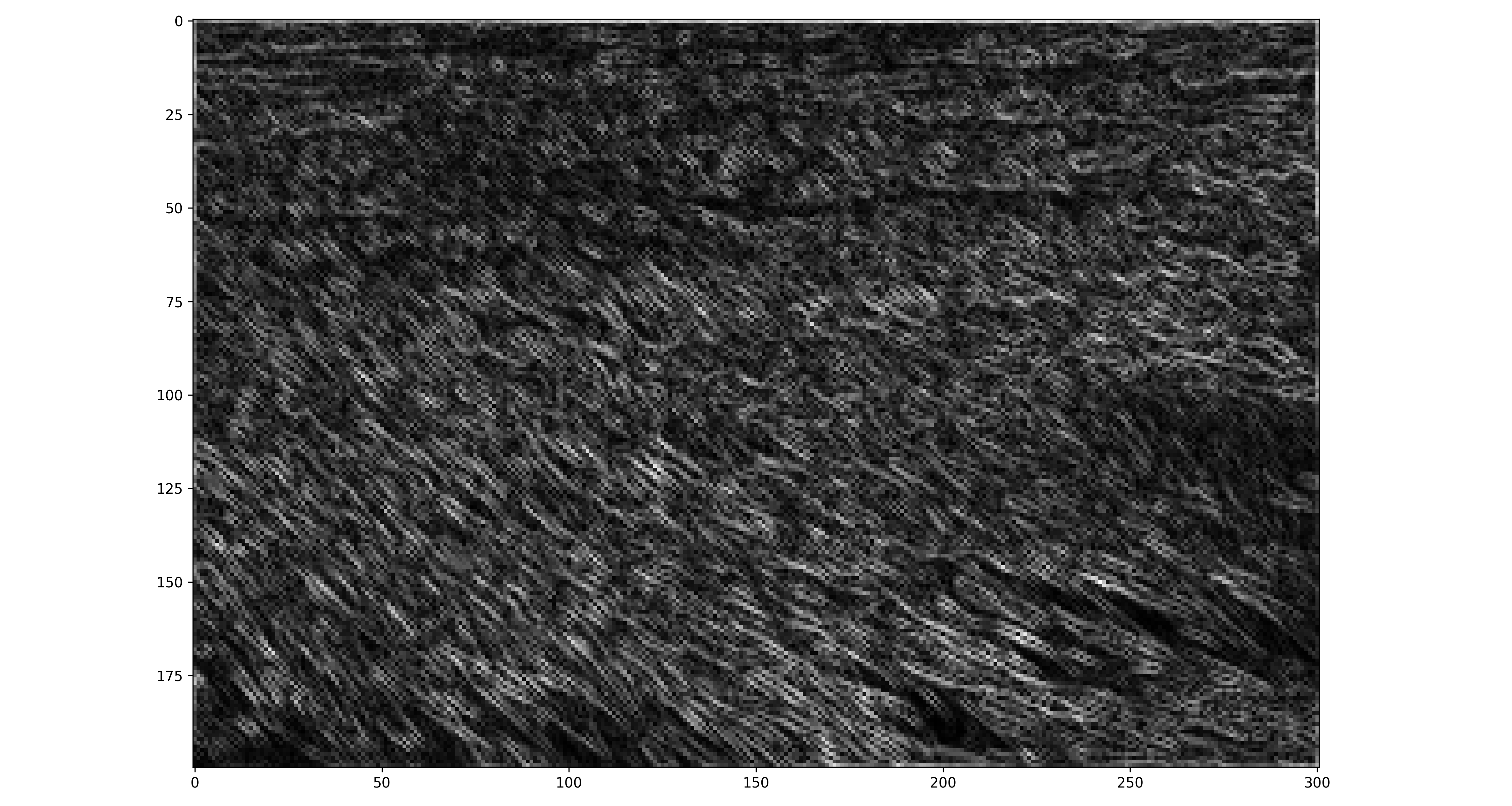
Create Data Frame for Each Image
Create Histograms of Gradient Magnitudes and Angles for Grass Images
Plot histogram of internet grass gradient magnitudes and define the magnitude level for later filtering
# Internet grass image histogram of gradient mags
internet_grass_histogram_mag_plot <-
  ggplot(grass_standard_df_list[[1]],
         aes(x = mag)) +
  geom_histogram(colour = "black", fill = "lightblue") +
  scale_x_continuous() +
  labs(x = "Gradient Magnitude",
       y = "Count",
       title = "Internet Grass Image Histogram of Gradient Magnitudes"
       ) +
  theme_minimal() +
  theme(plot.title = element_text(hjust = 0.5))

# Internet grass mag filter
internet_grass_mag_filter <- 0.3

# save image
ggsave("images/plots/grass/internet_grass_histogram_mag_plot.jpg",
       internet_grass_histogram_mag_plot,
       width = 6,
       height = 4,
       dpi = 300)
Plot histogram of internet grass gradient angles
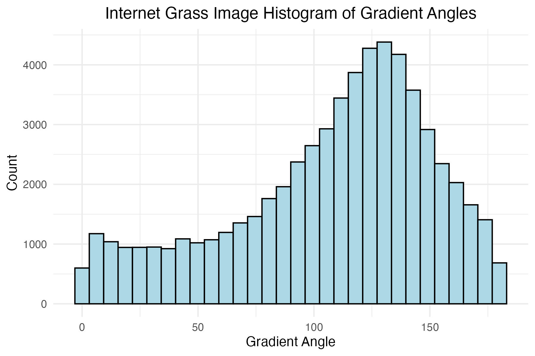
# Internet grass image histogram of gradient angles
internet_grass_histogram_theta_plot <-
ggplot(grass_standard_df_list[[1]],
aes(x = theta)) +
geom_histogram(colour = "black", fill = "lightblue") +
scale_x_continuous() +
labs(x = "Gradient Angle",
y = "Count",
title = "Internet Grass Image Histogram of Gradient Angles"
) +
theme_minimal() +
theme(plot.title = element_text(hjust = 0.5))
# save image
ggsave("images/plots/grass/internet_grass_histogram_theta_plot.jpg",
internet_grass_histogram_theta_plot,
width = 6,
height = 4,
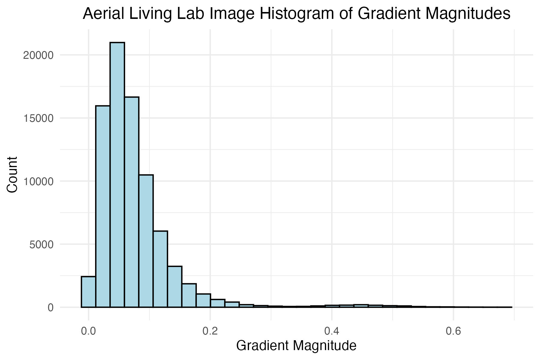
dpi = 300)Plot histogram of aerial Living Lab grass image gradient magnitudes and define the magnitude level for later filtering
# Aerial Living Lab image histogram of gradient mags
aerial_living_lab_histogram_mag_plot <-
  ggplot(grass_standard_df_list[[2]],
         aes(x = mag)) +
  geom_histogram(colour = "black", fill = "lightblue") +
  scale_x_continuous() +
  labs(x = "Gradient Magnitude",
       y = "Count",
       title = "Aerial Living Lab Image Histogram of Gradient Magnitudes"
  ) +
  theme_minimal() +
  theme(plot.title = element_text(hjust = 0.5))

# Aerial Living Lab mag filter
aerial_living_lab_mag_filter <- 0.08

# save image
ggsave("images/plots/grass/aerial_living_lab_histogram_mag_plot.jpg",
       aerial_living_lab_histogram_mag_plot,
       width = 6,
       height = 4,
       dpi = 300)
Plot histogram of aerial Living Lab grass image gradient angles
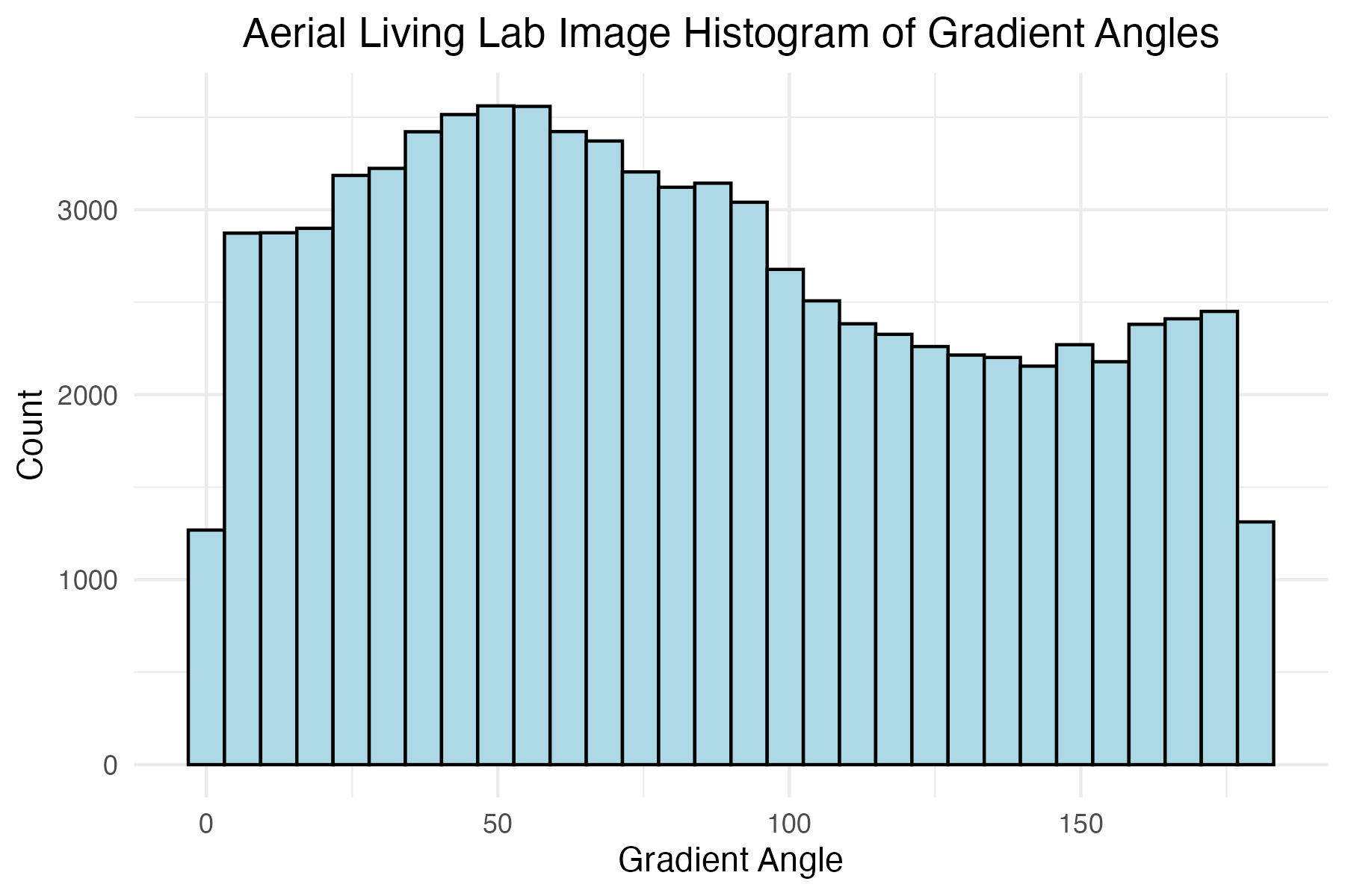
# Aerial Living Lab image histogram of gradient angles
aerial_living_lab_histogram_theta_plot <-
ggplot(grass_standard_df_list[[2]],
aes(x = theta)) +
geom_histogram(colour = "black", fill = "lightblue") +
scale_x_continuous() +
labs(x = "Gradient Angle",
y = "Count",
title = "Aerial Living Lab Image Histogram of Gradient Angles"
) +
theme_minimal() +
theme(plot.title = element_text(hjust = 0.5))
# save image
ggsave("images/plots/grass/aerial_living_lab_histogram_theta_plot.jpg",
aerial_living_lab_histogram_theta_plot,
width = 6,
height = 4,
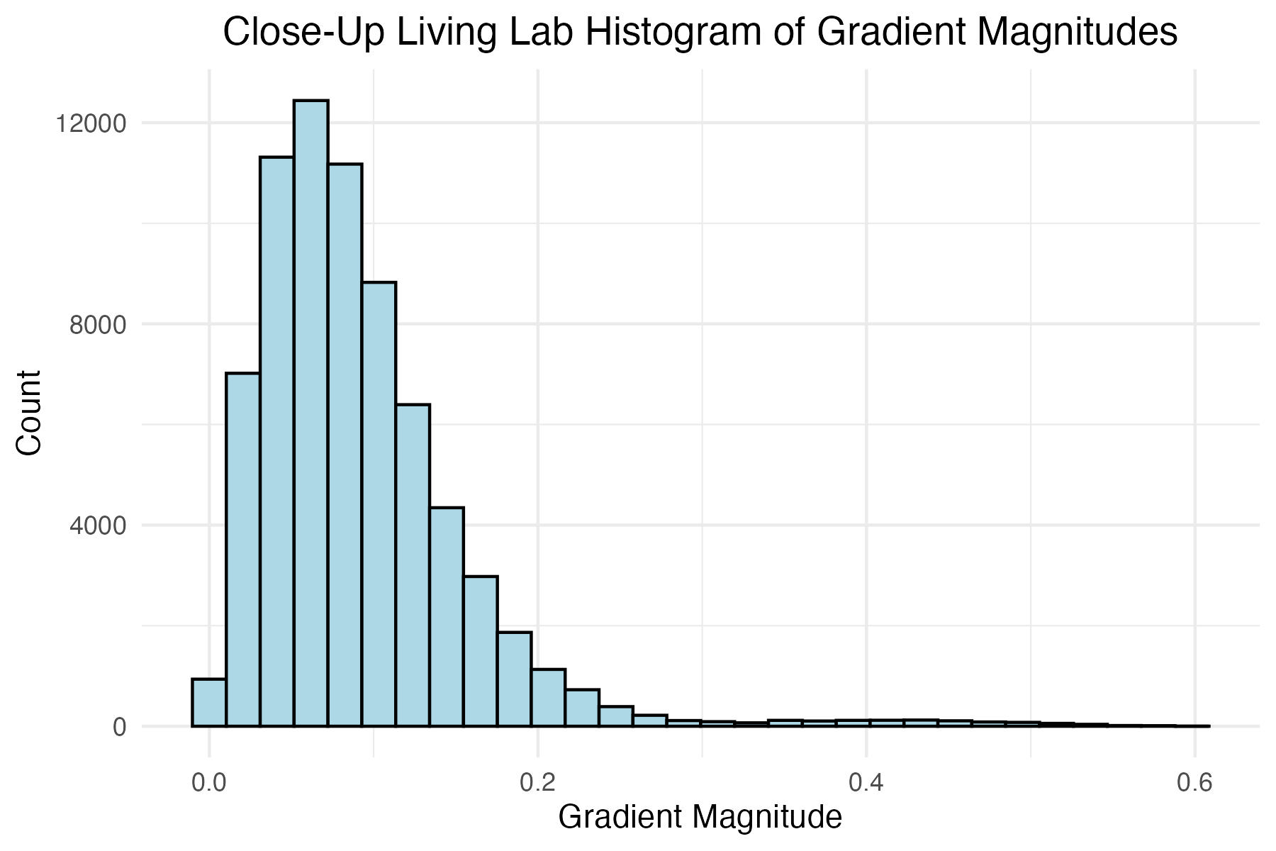
dpi = 300)Plot histogram of close-up Living Lab grass image gradient magnitudes and define the magnitude level for later filtering
# Close-up Living Lab image histogram of gradient mags
close_up_living_lab_histogram_mag_plot <-
  ggplot(grass_standard_df_list[[3]],
         aes(x = mag)) +
  geom_histogram(colour = "black", fill = "lightblue") +
  scale_x_continuous() +
  labs(x = "Gradient Magnitude",
       y = "Count",
       title = "Close-Up Living Lab Histogram of Gradient Magnitudes"
       ) +
  theme_minimal() +
  theme(plot.title = element_text(hjust = 0.5))

# Close-up mag filter
close_up_living_lab_mag_filter <- 0.12

# save image
ggsave("images/plots/grass/close_up_living_lab_histogram_mag_plot.jpg",
       close_up_living_lab_histogram_mag_plot,
       width = 6,
       height = 4,
       dpi = 300)
Plot histogram of close-up Living Lab grass image gradient angles
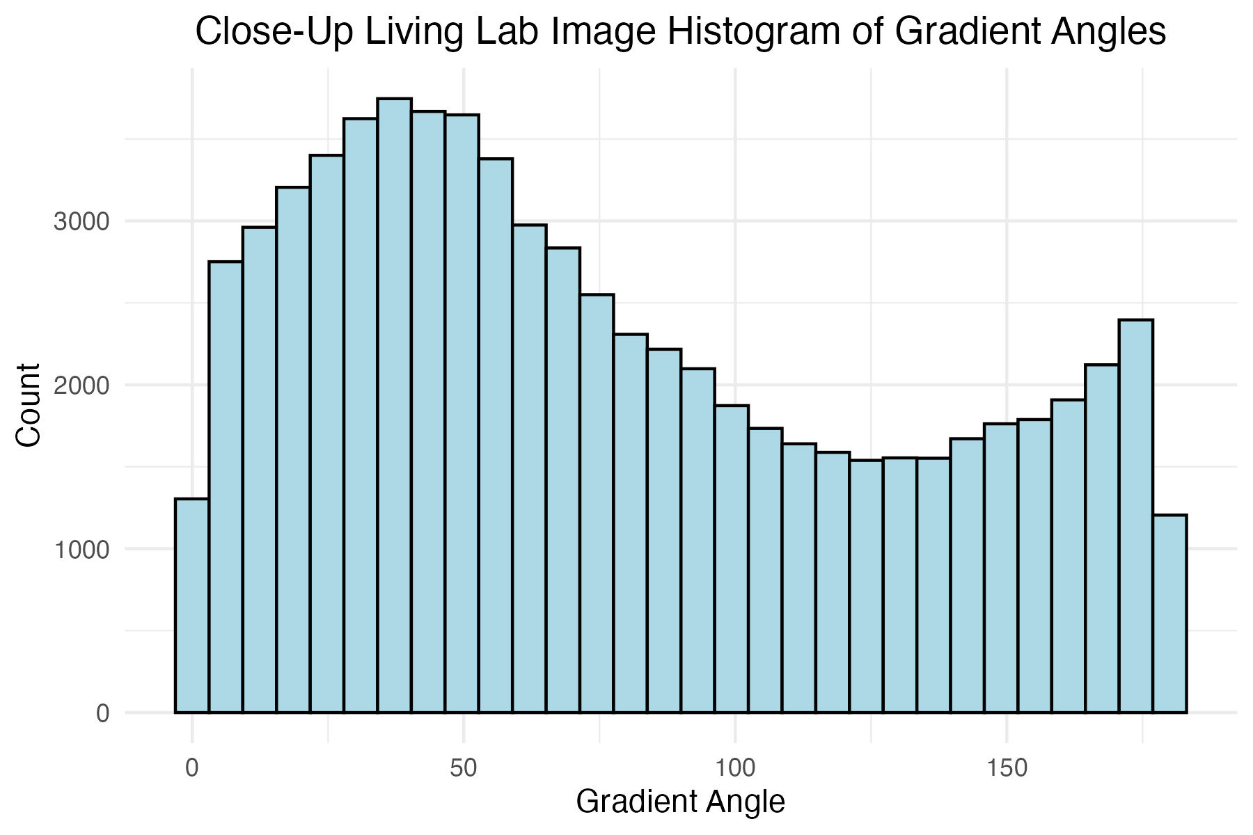
# Close-up Living Lab image histogram of gradient angles
close_up_living_lab_histogram_theta_plot <-
  ggplot(grass_standard_df_list[[3]],
         aes(x = theta)) +
  geom_histogram(colour = "black", fill = "lightblue") +
  scale_x_continuous() +
  labs(x = "Gradient Angle",
       y = "Count",
       title = "Close-Up Living Lab Image Histogram of Gradient Angles"
       ) +
  theme_minimal() +
  theme(plot.title = element_text(hjust = 0.5))

# save image
ggsave("images/plots/grass/close_up_living_lab_histogram_theta_plot.jpg",
       close_up_living_lab_histogram_theta_plot,
       width = 6,
       height = 4,
       dpi = 300)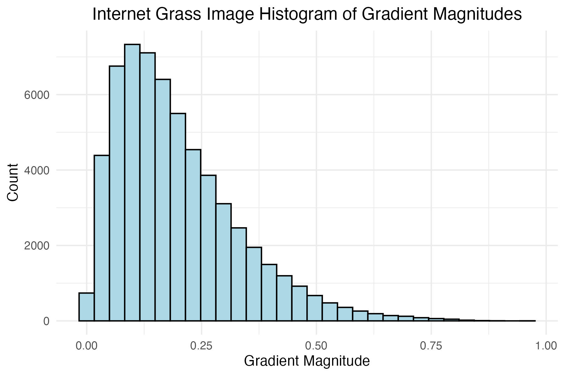
Build New Distributed Histogram Data Frames for Grass Images
Function for calculating values for each bin of distributed histogram
calculate_bin_contributions <- function(angle, magnitude, num_bins) {
  bin_width <- 180 / num_bins
  contributions <- numeric(num_bins)

  # get the central bin
  central_bin <- floor(angle / bin_width) %% num_bins
  next_bin <- (central_bin + 1) %% num_bins

  # get contributions to neighboring bins
  weight <- (1 - abs((angle %% bin_width) / bin_width)) * magnitude

  contributions[central_bin + 1] <- weight
  contributions[next_bin + 1] <- magnitude - weight

  return(list(contributions[1],
         contributions[2],
         contributions[3],
         contributions[4],
         contributions[5],
         contributions[6],
         contributions[7],
         contributions[8],
         contributions[9])
         )
}
Filter each data set of grass image gradients and angles to only contain observations with magnitudes greater than or equal to the respective magnitude levels determined above
# Create filtered data frames using the filter levels for
# magnitudes defined above, store all in a list
filtered_grass_standard_df_list <-
  list(internet_grass_hog_df %>%
         filter(mag >= internet_grass_mag_filter),
       aerial_living_lab_hog_df %>%
         filter(mag >= aerial_living_lab_mag_filter),
       close_up_living_lab_hog_df %>%
         filter(mag >= close_up_living_lab_mag_filter))
For each image calculate the contribution to each bin for the distribued histogram
# empty list for storing new distributed histogram data frames
grass_contribution_df_list <- list()

# Define the number of bins
num_bins <- 9

# iterate through each filtered standard data frame
for (i in 1:length(filtered_grass_standard_df_list)){

  grass_contribution_hog_df <-
    filtered_grass_standard_df_list[[i]] %>%
    rowwise() %>%
    mutate(`0` = calculate_bin_contributions(theta, mag, 9)[[1]],
           `20` = calculate_bin_contributions(theta, mag, 9)[[2]],
           `40` = calculate_bin_contributions(theta, mag, 9)[[3]],
           `60` = calculate_bin_contributions(theta, mag, 9)[[4]],
           `80` = calculate_bin_contributions(theta, mag, 9)[[5]],
           `100` = calculate_bin_contributions(theta, mag, 9)[[6]],
           `120` = calculate_bin_contributions(theta, mag, 9)[[7]],
           `140` = calculate_bin_contributions(theta, mag, 9)[[8]],
           `160` = calculate_bin_contributions(theta, mag, 9)[[9]],
           )

    # rearrange into same tidy format
  grass_split_histo_df <-
    grass_contribution_hog_df %>%
    pivot_longer(names_to = "bin",
                 values_to = "contribution",
                 cols = 4:ncol(grass_contribution_hog_df)) %>%
    mutate(bin = as.numeric(bin)) %>%
    group_by(bin) %>%
    summarise(contribution_sum = sum(contribution))

  # add to list for storage
  grass_contribution_df_list[[i]] <- grass_split_histo_df

}
Generate Polar Plots for Images Using Standard Histogram Binning Technique
Polar plot of internet grass histogram of gradient angles using standard binning technique
# Internet grass plot
internet_grass_plot <-
ggplot(filtered_grass_standard_df_list[[1]],
aes(x = theta)) +
geom_histogram(colour = "black",
fill = "lightblue",
breaks = seq(0, 360, length.out = 17.5),
bins = 9) +
coord_polar(
theta = "x",
start = 0,
direction = 1) +
scale_x_continuous(limits = c(0,360),
breaks = c(0, 45, 90, 135, 180, 225, 270, 315),
labels = c("N", "NE", "E", "SE", "S", "SW", "W", "NW")
)+
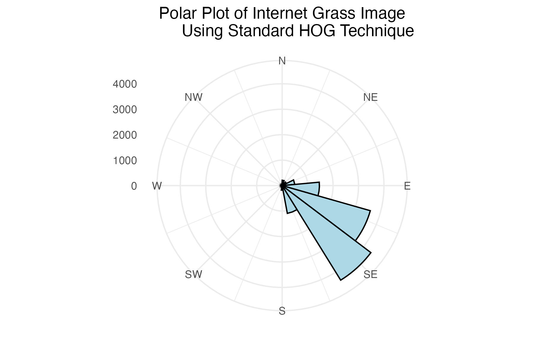
labs(title = "Polar Plot of Internet Grass Image
Using Standard HOG Technique") +
theme_minimal() +
labs(x = "") +
theme(axis.title.y = element_blank(),
plot.title = element_text(hjust = 0.5))
# save image
ggsave("images/plots/grass/internet_grass_standard_polar_plot.jpg",
internet_grass_plot,
width = 6,
height = 4,
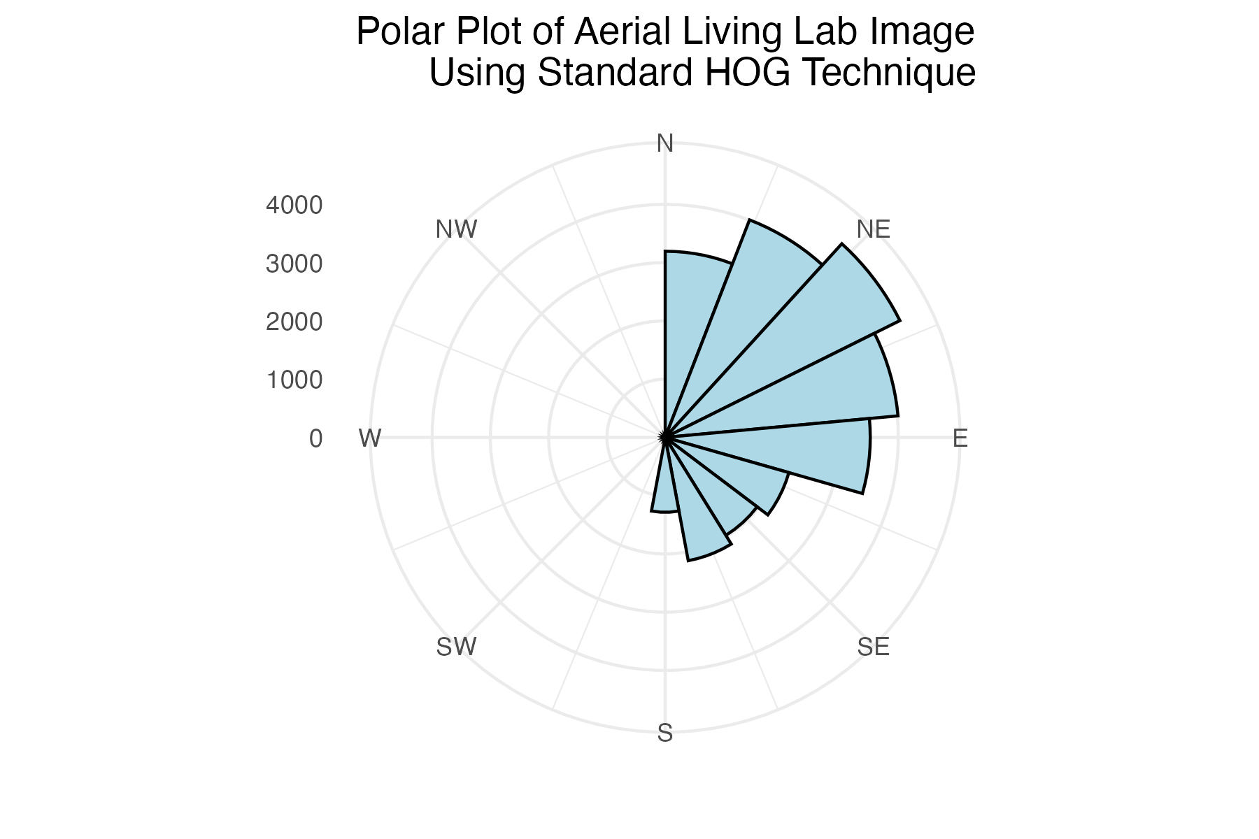
dpi = 300)Polar plot of aerial Living Lab histogram of gradient angles using standard binning technique
# Aerial Living Lab plot
aerial_living_lab_plot <-
ggplot(filtered_grass_standard_df_list[[2]],
aes(x = theta)) +
geom_histogram(colour = "black",
fill = "lightblue",
breaks = seq(0, 360, length.out = 17.5),
bins = 9) +
coord_polar(
theta = "x",
start = 0,
direction = 1) +
scale_x_continuous(limits = c(0,360),
breaks = c(0, 45, 90, 135, 180, 225, 270, 315),
labels = c("N", "NE", "E", "SE", "S", "SW", "W", "NW")
)+
labs(title = "Polar Plot of Aerial Living Lab Image
Using Standard HOG Technique") +
theme_minimal() +
labs(x = "") +
theme(axis.title.y = element_blank(),
plot.title = element_text(hjust = 0.5))
# save image
ggsave("images/plots/grass/aerial_living_lab_standard_polar_plot.jpg",
aerial_living_lab_plot,
width = 6,
height = 4,
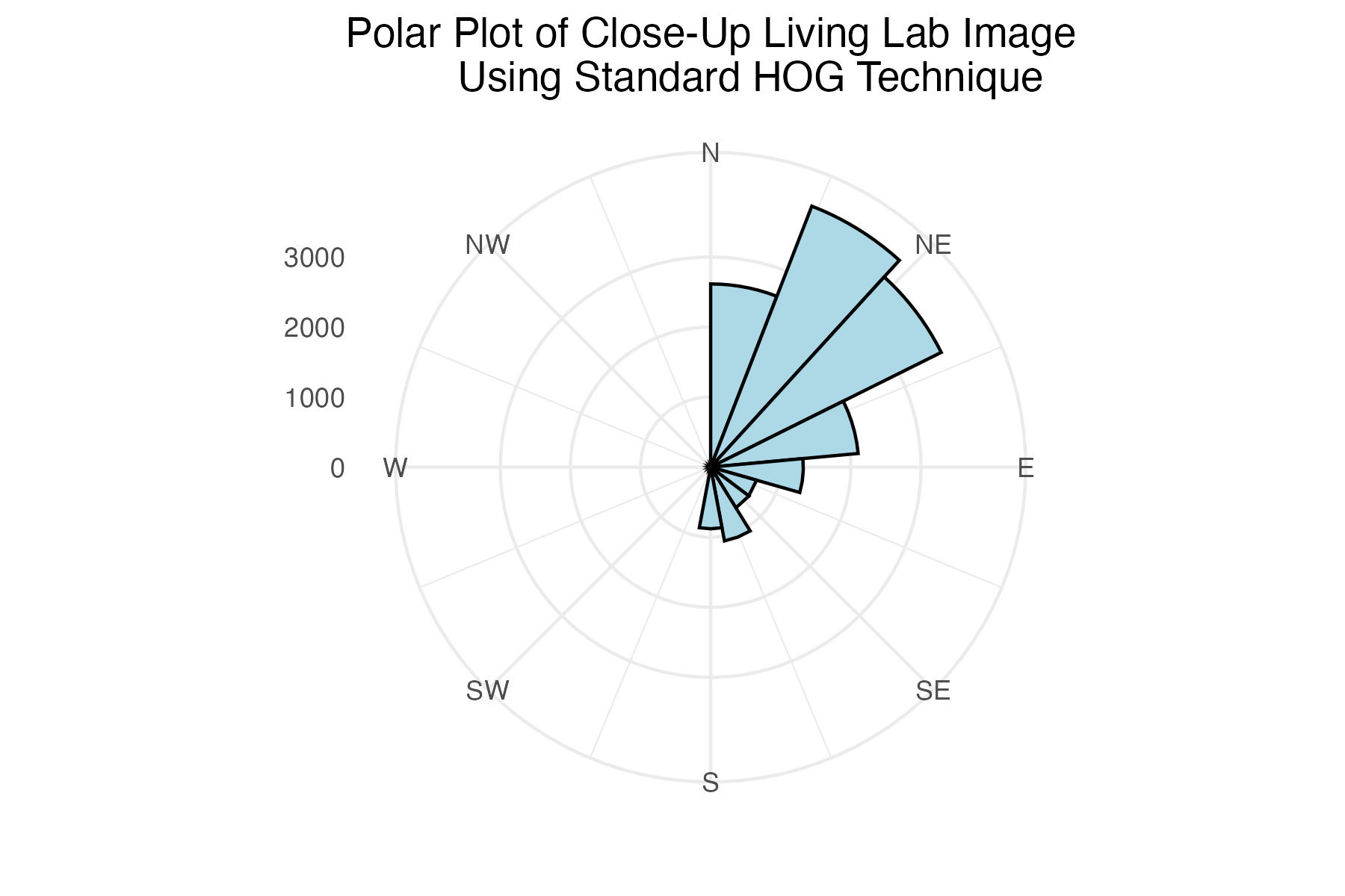
dpi = 300)Polar plot of close-up Living Lab histogram of gradient angles using standard binning technique
# Close-up Living Lab plot
close_up_living_lab_plot <-
  ggplot(filtered_grass_standard_df_list[[3]],
         aes(x = theta)) +
  geom_histogram(colour = "black",
                 fill = "lightblue",
                 breaks = seq(0, 360, length.out = 17.5),
                 bins = 9) +
  coord_polar(
    theta = "x",
    start = 0,
    direction = 1) +
  scale_x_continuous(limits = c(0,360),
    breaks = c(0, 45, 90, 135, 180, 225, 270, 315),
    labels = c("N", "NE", "E", "SE", "S", "SW", "W", "NW")
  )+
  labs(title = "Polar Plot of Close-Up Living Lab Image
       Using Standard HOG Technique") +
  theme_minimal() +
  labs(x = "") +
  theme(axis.title.y = element_blank(),
        plot.title = element_text(hjust = 0.5))

# save image
ggsave("images/plots/grass/close_up_living_lab_standard_polar_plot.jpg",
       close_up_living_lab_plot,
       width = 6,
       height = 4,
       dpi = 300)
Save an arranged image of the 3 plots side-by-side
Generate Polar Plots for Images Using Distributed Histogram Binning Technique
Polar plot of internet grass histogram of gradient angles using distributed binning technique
# Internet grass plot
internet_grass_split_plot <-
  ggplot(grass_contribution_df_list[[1]],
         aes(x = bin, y = contribution_sum)) +
  geom_histogram(stat = "identity",
                 colour = "black",
                 fill = "lightblue",
                 breaks = seq(0, 360, length.out = 17.5),
                 bins = 9) +
  coord_polar(
    theta = "x",
    start = 0,
    direction = 1) +
  scale_x_continuous(limits = c(0,360),
    breaks = c(0, 45, 90, 135, 180, 225, 270, 315),
    labels = c("N", "NE", "E", "SE", "S", "SW", "W", "NW")
  )+
  labs(title = "Polar Plot of Internet Grass Image
       Using Distributed HOG Technique") +
  theme_minimal() +
  labs(x = "") +
  theme(axis.title.y = element_blank(),
        plot.title = element_text(hjust = 0.5))

# save image
ggsave("images/plots/grass/internet_grass_contribution_polar_plot.jpg",
       internet_grass_split_plot,
       width = 6,
       height = 4,
       dpi = 300)
Polar plot of aerial Living Lab histogram of gradient angles using distributed binning technique
# Aerial Living Lab plot
aerial_living_lab_split_plot <-
  ggplot(grass_contribution_df_list[[2]],
         aes(x = bin, y = contribution_sum)) +
  geom_histogram(stat = "identity",
                 colour = "black",
                 fill = "lightblue",
                 breaks = seq(0, 360, length.out = 17.5),
                 bins = 9) +
  coord_polar(
    theta = "x",
    start = 0,
    direction = 1) +
  scale_x_continuous(limits = c(0,360),
    breaks = c(0, 45, 90, 135, 180, 225, 270, 315),
    labels = c("N", "NE", "E", "SE", "S", "SW", "W", "NW")
  )+
  labs(title = "Polar Plot of Aerial Living Lab Image
       Using Distributed HOG Technique") +
  theme_minimal() +
  labs(x = "") +
  theme(axis.title.y = element_blank(),
        plot.title = element_text(hjust = 0.5))

# save image
ggsave("images/plots/grass/aerial_living_lab_contribution_polar_plot.jpg",
       aerial_living_lab_split_plot,
       width = 6,
       height = 4,
       dpi = 300)
Polar plot of close-up Living Lab histogram of gradient angles using distributed binning technique
# Close-up Living Lab plot
close_up_living_lab_split_plot <-
  ggplot(grass_contribution_df_list[[3]],
         aes(x = bin, y = contribution_sum)) +
  geom_histogram(stat = "identity",
                 colour = "black",
                 fill = "lightblue",
                 breaks = seq(0, 360, length.out = 17.5),
                 bins = 9) +
  coord_polar(
    theta = "x",
    start = 0,
    direction = 1) +
  scale_x_continuous(limits = c(0,360),
    breaks = c(0, 45, 90, 135, 180, 225, 270, 315),
    labels = c("N", "NE", "E", "SE", "S", "SW", "W", "NW")
  )+
  labs(title = "Polar Plot of Close-Up Living Lab Image
       Using Distributed HOG Technique") +
  theme_minimal() +
  labs(x = "") +
  theme(axis.title.y = element_blank(),
        plot.title = element_text(hjust = 0.5))

# save image
ggsave("images/plots/grass/close_up_living_lab_contribution_polar_plot.jpg",
       close_up_living_lab_split_plot,
       width = 6,
       height = 4,
       dpi = 300)
Save an arranged image of the 3 distributed-binned polar plots side-by-side
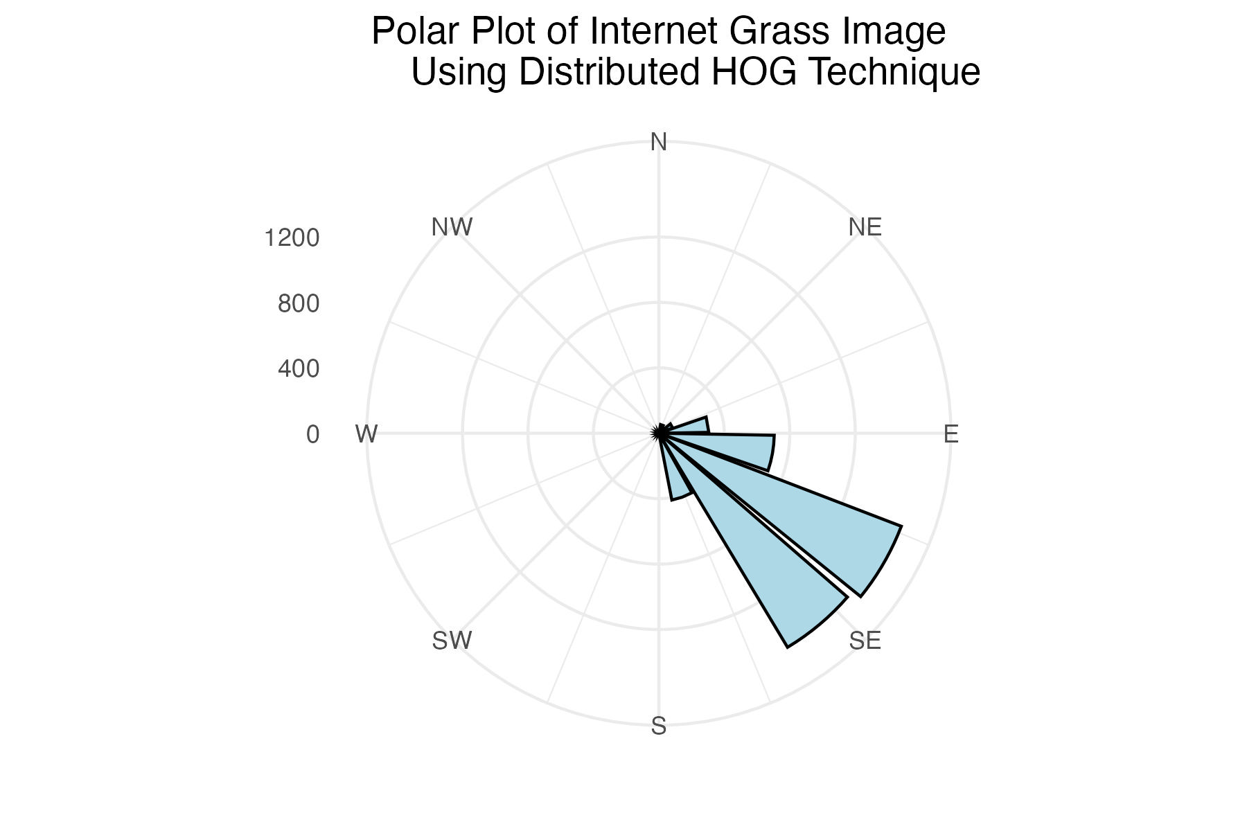
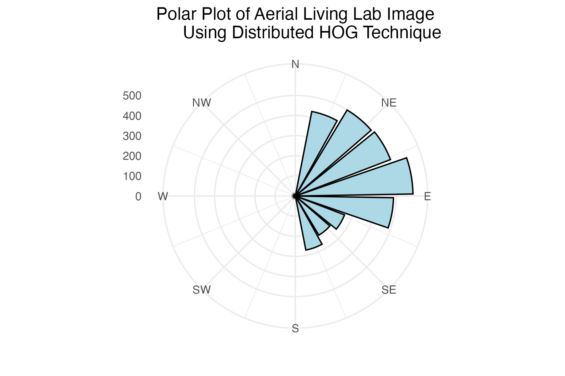

Discussion
The internet grass image was selected for its simplicity and general diagonal direction. Both techniques proved quite successful at identifying the image’s predominate diagonal gradient angles. The aerial image from the Living Laboratory posed a greater challenge due to its wider zoom range, causing a higher degree of variability in grass lay direction. Ultimately, the standard binning technique was able to identify this north-eastern trend seen on the right side of the image, while the distributed method identified a slightly more eastern trend. Lastly, the north-eastern trend in close-up image from the Living Laboratory was successfully identified in both the standard and distributed methods of binning.