3 Methods
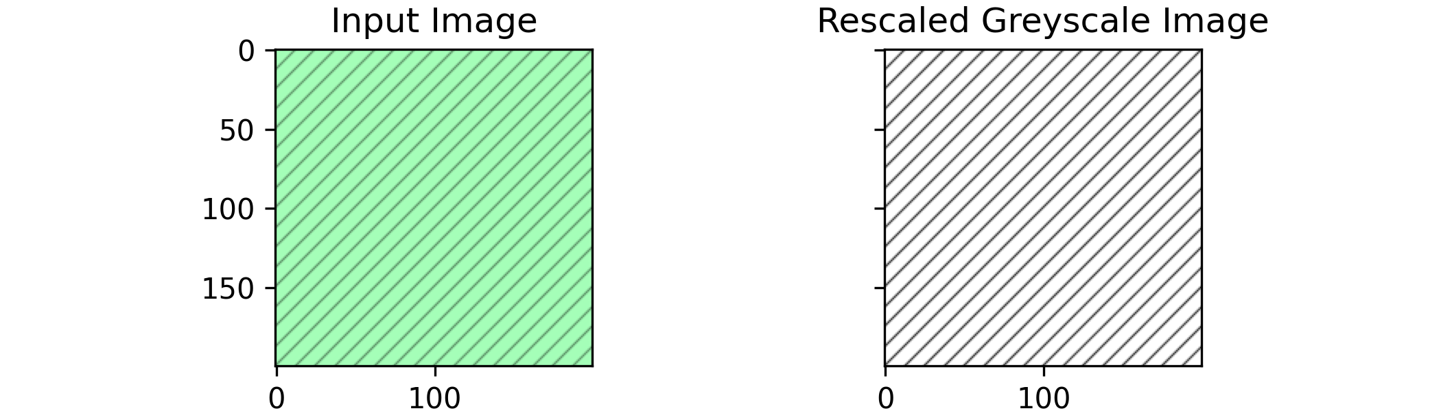
The HOG algorithm, introduced by Navneet Dalal and Bill Triggs in 2005 (Dalal and Triggs 2005), is a popular technique for object detection in images. The algorithm can identify gradient magnitudes and angles at each pixel in an image. The preliminary steps involved using the ‘skimage’ library from Python to preprocess the images of interest. This included loading, resizing, and converting the images to grayscale. Images were rescaled to standardize their resolutions and preserve their aspect ratios to prevent distortion that could affect the accuracy of angle identification. Converting the images to grayscale was necessary because it allowed for focusing on a single channel to represent pixel intensity, rather than three channels (red, green, and blue).
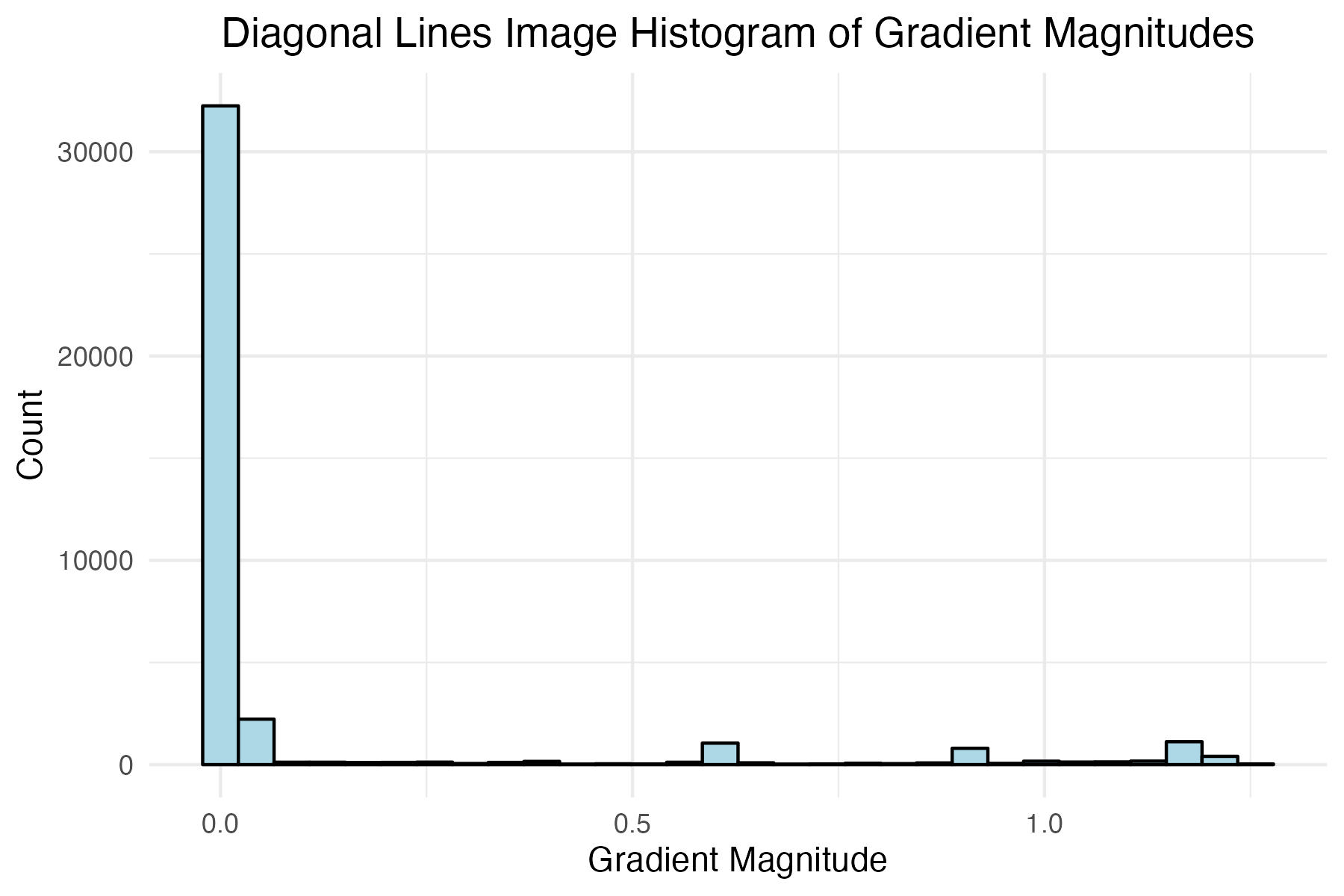
The HOG features were then computed for the resized images, which involved calculating the gradient magnitudes and angles at each pixel. The gradient magnitude at each pixel is comprised of the gradients in the ‘x’ and ‘y’ directions. The gradient in the x-direction is computed by subtracting the pixel value to the left of pixel of interest from the pixel value to its right. Similarly, the gradient in the y-direction is calculated by subtracting the pixel value below the pixel of interest from the pixel value above the pixel of interest.
\(G_x=I(r,c+1)−I(r,c-1)\)
\(G_y=I(r+1,c)−I(r-1,c)\)
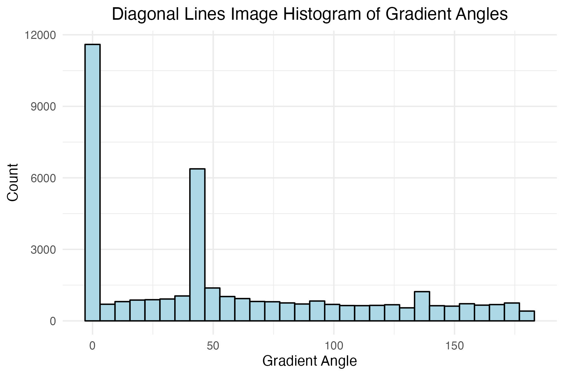
Now to calculate the gradient magnitude at the pixel of interest, the Pythagorean Theorem can be utilized where the gradient magnitude is equal to the square root of the x-gradient squared plus the y-gradient squared. The angle at a given pixel can be calculated by taking the inverse tangent of its y-gradient divided by its x-gradient. It is important to note all angles produced by this algorithm are between zero and one hundred eighty degrees. This occurs, because the inverse tangent function used for calculating a given pixel’s angle cannot distinguish between all four quadrants.
\(Magnitude(\mu)=\sqrt{G_{x}^{2} + G_{y}^{2}}\)
\(Angle(\Theta)=tan^{−1} (\frac{G_y}{G_x})\)
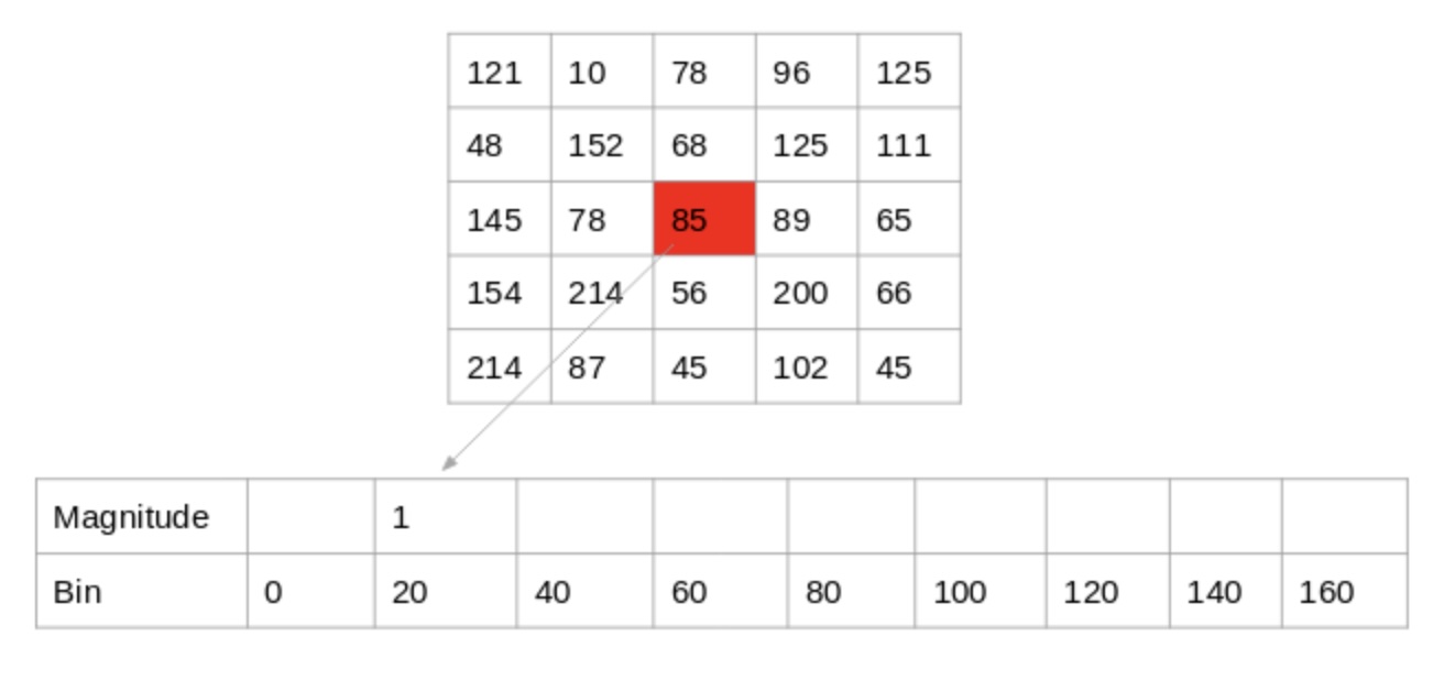
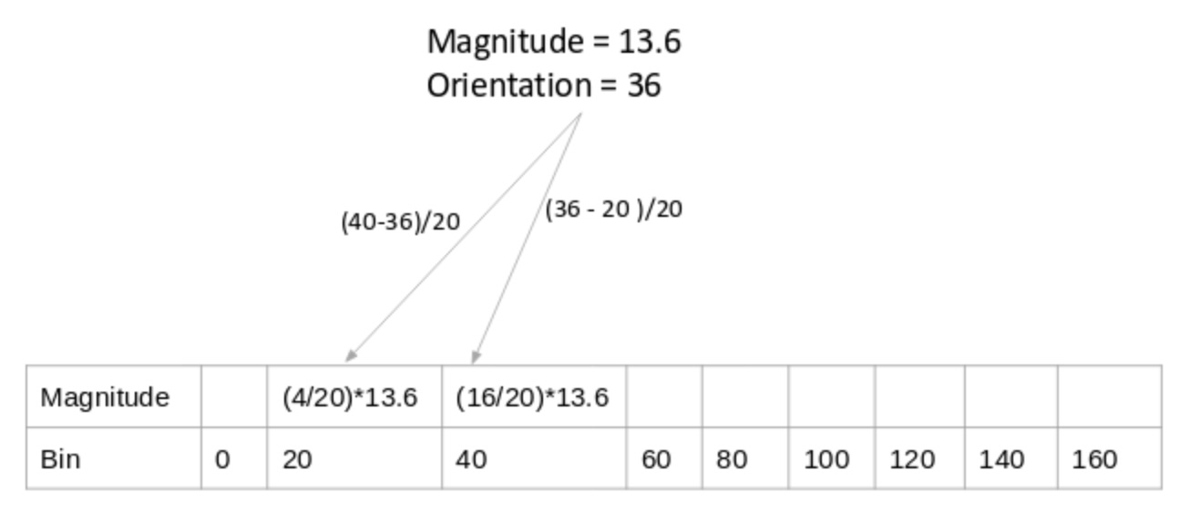
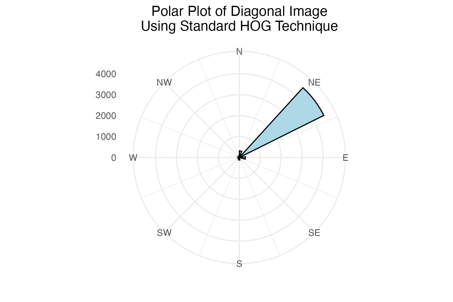
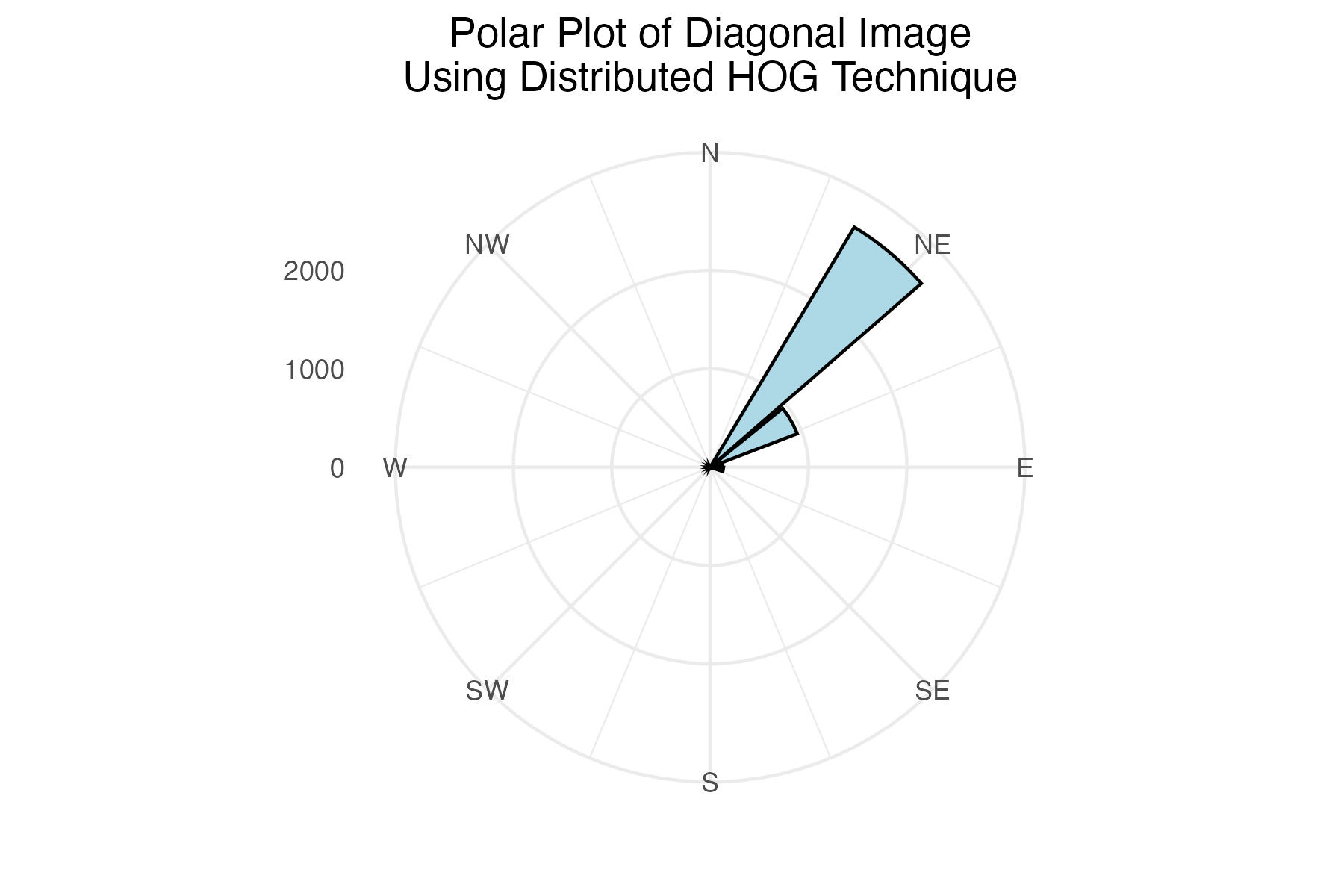
Next, histograms are constructed to visualize the distribution of gradient magnitudes and angles. Two different techniques for creating gradient angle histograms were implemented. The first histogram was created by counting the number of angles that fell into their respective bins. The second scheme factors in a pixel’s gradient magnitude and its allocation to its bordering bins. Here, the weight assigned to each bin is calculated by the angle’s deviation from the center of its central bin. This approach allows for a more representative histogram which splits angles between bins and takes their magnitudes into account. Lastly, these histograms are converted to polar histograms so the primary angles can be visualized and compared to their original images.
References
Dalal, N., and B. Triggs. 2005. “Histograms of Oriented Gradients for Human Detection.” In 2005 IEEE Computer Society Conference on Computer Vision and Pattern Recognition (CVPR’05), 1:886–893 vol. 1. https://doi.org/10.1109/CVPR.2005.177.
Singh, Aishwarya. 2024. “Feature Engineering for Images: A Valuable Introduction to the Hog Feature Descriptor.” Analytics Vidhya. https://www.analyticsvidhya.com/blog/2019/09/feature-engineering-images-introduction-hog-feature-descriptor/.