6 Backflip Image
Motivation
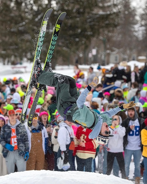
Test the HOG algorithm’s ability to identify dominant edges using an image of a skier. This scenario adds complexity with both a skier in the foreground and a crowd in the background, allowing us to observe how the algorithm deals with additional “noise”.
Input Image
Load R Packages and Python Libraries
Code
# Load Python Libraries
import matplotlib.pyplot as plt
import pandas as pd
from skimage.io import imread, imshow
from skimage.transform import resize
from skimage.feature import hog
from skimage import data, exposure
import matplotlib.pyplot as plt
from skimage import io
from skimage import color
from skimage.transform import resize
import math
from skimage.feature import hog
import numpy as np
Collect HOG Features for Backflip Image
Code
# List for storing images
img_list = []

# SF aerial
img_list.append(color.rgb2gray(io.imread("images/TitusFlip.jpg")))

# List to store magnitudes for each image
mag_list = []

# List to store angles for each image
theta_list = []


for x in range(len(img_list)):
    # Get image of interest
    img = img_list[x]

    rescaled_file_path = f"images/plots/backflip/{x}.jpg"

    # Determine aspect Ratio
    aspect_ratio = img.shape[0] / img.shape[1]
    print("Aspect Ratio:", aspect_ratio)

    # Hard-Code height to 200 pixels
    height = 200

    # Calculate witdth to maintain same aspect ratio
    width = int(height / aspect_ratio)
    print("Resized Width:", width)

    # Resize the image
    resized_img = resize(img, (height, width))

    # Replace the original image with the resized image
    img_list[x] = resized_img

    # plt.figure(figsize=(15, 8))
    # plt.imshow(resized_img, cmap="gray")
    # plt.axis("on")
    # plt.tight_layout()
    # plt.savefig(rescaled_file_path, dpi=300)
    # plt.show()

    # list for storing all magnitudes for image[x]
    mag = []

    # list for storing all angles for image[x]
    theta = []

    for i in range(height):
        magnitudeArray = []
        angleArray = []

        for j in range(width):
            if j - 1 < 0 or j + 1 >= width:
                if j - 1 < 0:
                    Gx = resized_img[i][j + 1] - 0
                elif j + 1 >= width:
                    Gx = 0 - resized_img[i][j - 1]
            else:
                Gx = resized_img[i][j + 1] - resized_img[i][j - 1]

            if i - 1 < 0 or i + 1 >= height:
                if i - 1 < 0:
                    Gy = 0 - resized_img[i + 1][j]
                elif i + 1 >= height:
                    Gy = resized_img[i - 1][j] - 0
            else:
                Gy = resized_img[i + 1][j] - resized_img[i - 1][j]

            magnitude = math.sqrt(pow(Gx, 2) + pow(Gy, 2))
            magnitudeArray.append(round(magnitude, 9))

            if Gx == 0:
                angle = math.degrees(0.0)
            else:
                angle = math.degrees(math.atan(Gy / Gx))
                if angle < 0:
                    angle += 180

            angleArray.append(round(angle, 9))

        mag.append(magnitudeArray)
        theta.append(angleArray)

    # add list of magnitudes to list[x]
    mag_list.append(mag)

    # add list of angles to angle list[x]
    theta_list.append(theta)
Aspect Ratio: 1.25
Resized Width: 160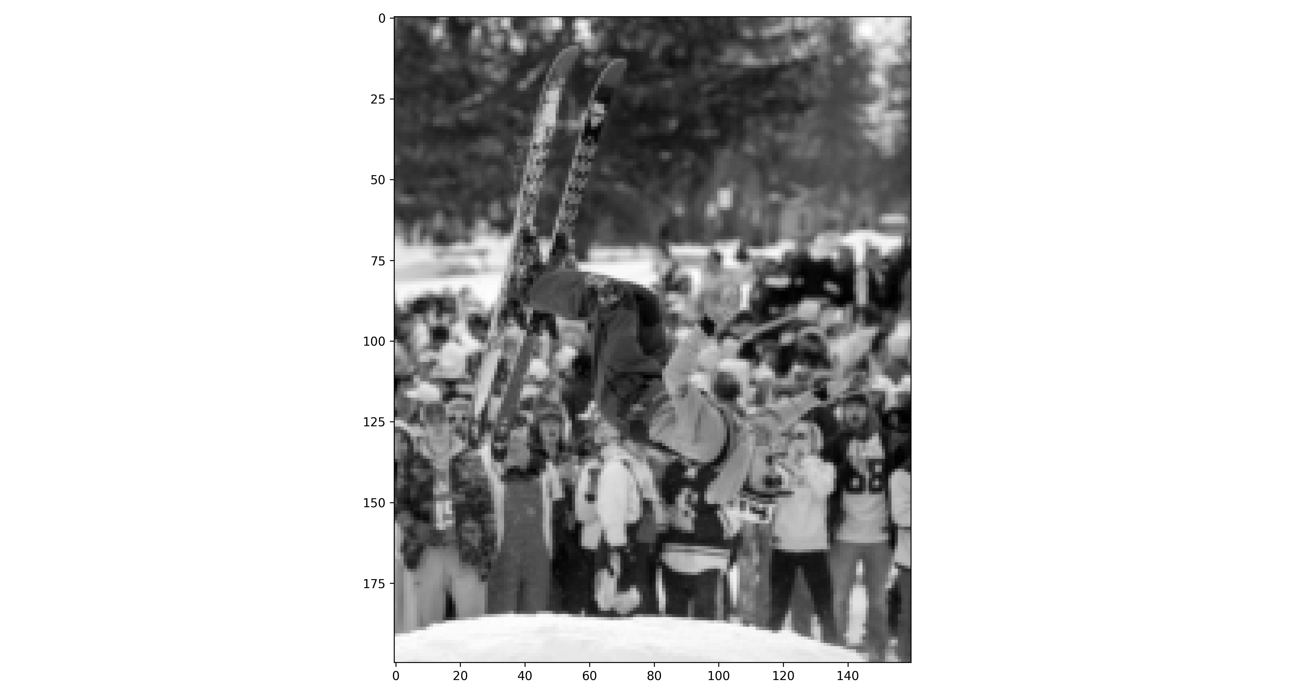
Extract Gradient Magnitudes and Angles from Backflip Image
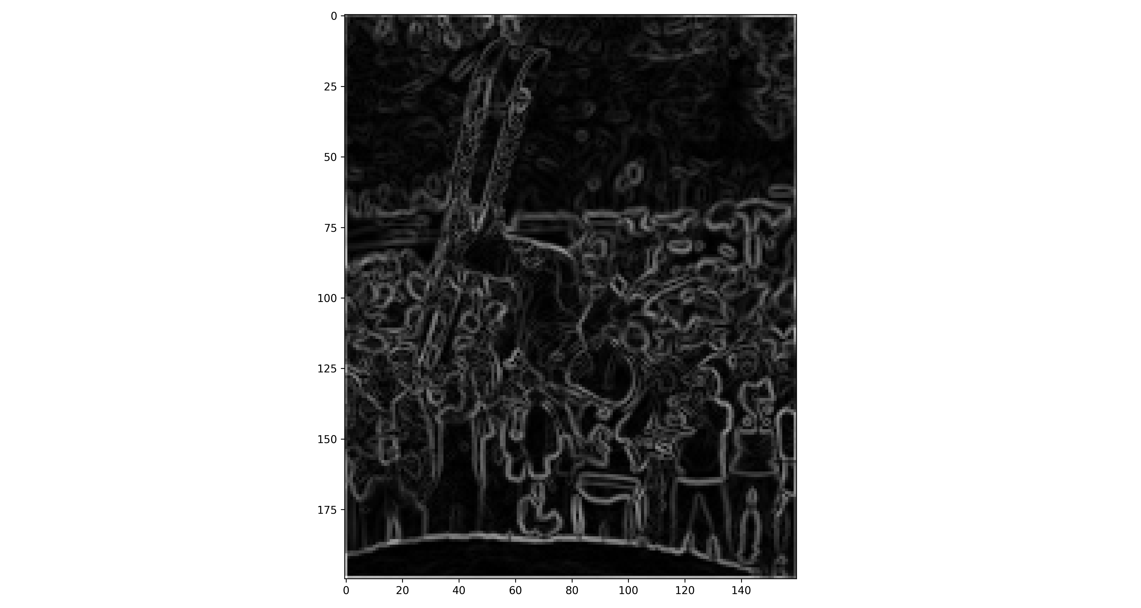
Plot Gradient Magnitudes as Image for Backflip Image
Create Data Frame for Backflip Image
Create Histograms of Gradient Magnitudes and Angles for Backflip Image
Plot histogram of backflip image gradient magnitudes and define the magnitude level for later filtering
# backflip histogram of gradient mags
flip_histogram_mag_plot <-
  ggplot(flip_standard_df_list[[1]],
         aes(x = mag)) +
  geom_histogram(colour = "black", fill = "lightblue") +
  scale_x_continuous() +
  labs(x = "Gradient Magnitude",
       y = "Count",
       title = "Skiing Backflip Image Histogram of Gradient Magnitudes"
       ) +
  theme_minimal() +
  theme(plot.title = element_text(hjust = 0.5))

# flip magn filter level
flip_mag_filter <- 0.2

# save image
ggsave("images/plots/backflip/backflip_histogram_mag_plot.jpg",
       flip_histogram_mag_plot,
       width = 6,
       height = 4,
       dpi = 300)
Plot histogram of backflip image gradient angles
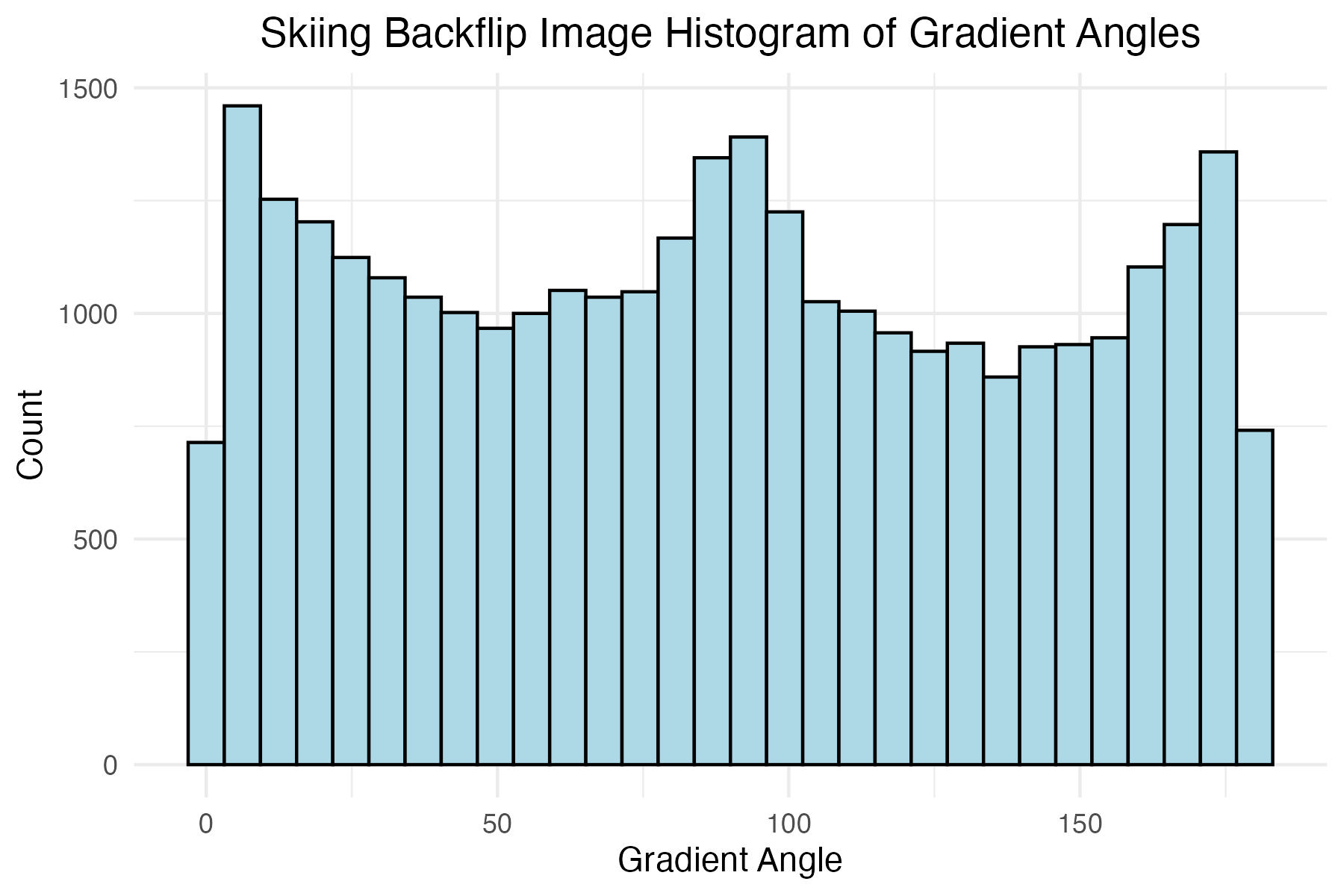
# backflip histogram of gradient angles
flip_histogram_theta_plot <-
  ggplot(flip_standard_df_list[[1]],
         aes(x = theta)) +
  geom_histogram(colour = "black", fill = "lightblue") +
  scale_x_continuous() +
  labs(x = "Gradient Angle",
       y = "Count",
       title = "Skiing Backflip Image Histogram of Gradient Angles"
       ) +
  theme_minimal() +
  theme(plot.title = element_text(hjust = 0.5))

# save image
ggsave("images/plots/backflip/backflip_histogram_theta_plot.jpg",
       flip_histogram_theta_plot,
       width = 6,
       height = 4,
       dpi = 300)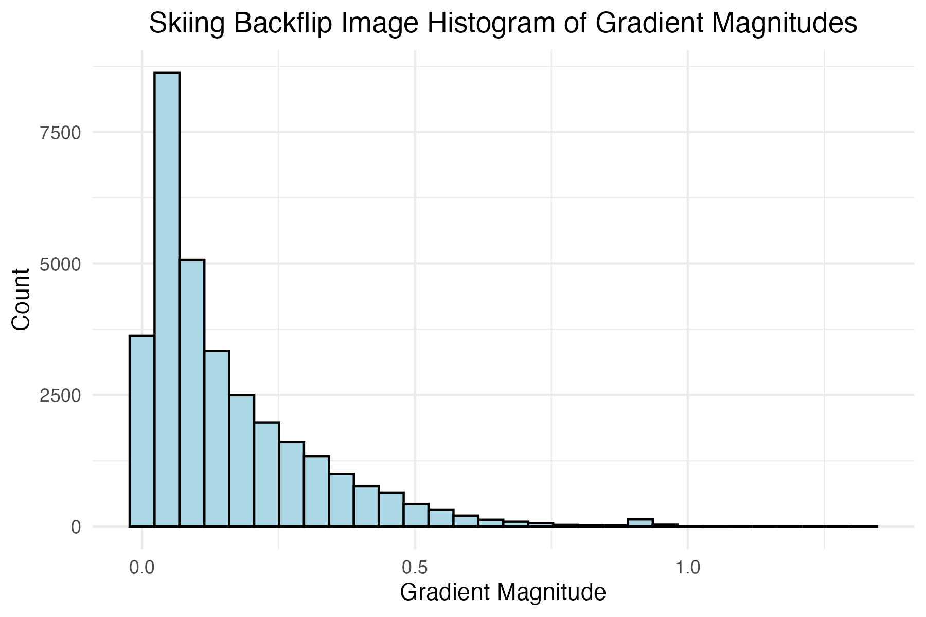
Build New Distributed Histogram Data Frame for Backflip Image
Function for calculating values for each bin of distributed histogram
# function to calculate the contributions to neighboring bins
calculate_bin_contributions <- function(angle, magnitude, num_bins) {
  bin_width <- 180 / num_bins
  contributions <- numeric(num_bins)

  # get the central bin
  central_bin <- floor(angle / bin_width) %% num_bins
  next_bin <- (central_bin + 1) %% num_bins

  # get contributions to neighboring bins
  weight <- (1 - abs((angle %% bin_width) / bin_width)) * magnitude

  contributions[central_bin + 1] <- weight
  contributions[next_bin + 1] <- magnitude - weight

  return(list(contributions[1],
         contributions[2],
         contributions[3],
         contributions[4],
         contributions[5],
         contributions[6],
         contributions[7],
         contributions[8],
         contributions[9])
         )
}
Filter data frame of gradients and angles to only contain observations with magnitudes greater than or equal to the respective magnitude levels determined above
Calculate the contribution to each bin for the distribued histogram
# Define the number of bins
num_bins <- 9
flip_contribution_df_list <- list()

# iterate through each filtered standard data frame (only 1 in this case)
for (i in 1:length(filtered_flip_standard_df_list)){

  flip_contribution_hog_df <-
    filtered_flip_standard_df_list[[i]] %>%
    rowwise() %>%
    mutate(`0` = calculate_bin_contributions(theta, mag, 9)[[1]],
           `20` = calculate_bin_contributions(theta, mag, 9)[[2]],
           `40` = calculate_bin_contributions(theta, mag, 9)[[3]],
           `60` = calculate_bin_contributions(theta, mag, 9)[[4]],
           `80` = calculate_bin_contributions(theta, mag, 9)[[5]],
           `100` = calculate_bin_contributions(theta, mag, 9)[[6]],
           `120` = calculate_bin_contributions(theta, mag, 9)[[7]],
           `140` = calculate_bin_contributions(theta, mag, 9)[[8]],
           `160` = calculate_bin_contributions(theta, mag, 9)[[9]],
           )

  # rearrange into same tidy format
  flip_split_histo_df <-
    flip_contribution_hog_df %>%
    pivot_longer(names_to = "bin",
                 values_to = "contribution",
                 cols = 4:ncol(flip_contribution_hog_df)) %>%
    mutate(bin = as.numeric(bin)) %>%
    group_by(bin) %>%
    summarise(contribution_sum = sum(contribution))

  # add to list for storage
  flip_contribution_df_list[[i]] <- flip_split_histo_df

}
Generate Polar Plots for Standard Histograms for Backflip Image
Polar plot of backflip image histogram of gradient angles using standard binning technique
# backflip plot
flip_plot <-
  ggplot(filtered_flip_standard_df_list[[1]],
         aes(x = theta)) +
  geom_histogram(colour = "black",
                 fill = "lightblue",
                 breaks = seq(0, 360, length.out = 17.5),
                 bins = 9) +
  coord_polar(
    theta = "x",
    start = 0,
    direction = 1) +
  scale_x_continuous(limits = c(0,360),
    breaks = c(0, 45, 90, 135, 180, 225, 270, 315),
    labels = c("N", "NE", "E", "SE", "S", "SW", "W", "NW")
  )+
  labs(title = "Polar Plot of Skiing Backflip
       Image Using Standard HOG Technique") +
  theme_minimal() +
  labs(x = "") +
  theme(axis.title.y = element_blank(),
        plot.title = element_text(hjust = 0.5))

# save image
ggsave("images/plots/backflip/backflip_standard_polar_plot.jpg",
       flip_plot,
       width = 6,
       height = 4,
       dpi = 300)
Generate Polar Plots for Distributed Histograms for Backflip Image
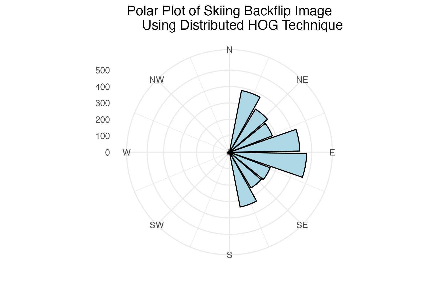
Polar plot of backflip image histogram of gradient angles using distributed binning technique
# backflip plot
flip_split_plot <-
  ggplot(flip_contribution_df_list[[1]],
         aes(x = bin, y = contribution_sum)) +
  geom_histogram(stat = "identity",
                 colour = "black",
                 fill = "lightblue",
                 breaks = seq(0, 360, length.out = 17.5),
                 bins = 9) +
  coord_polar(
    theta = "x",
    start = 0,
    direction = 1) +
  scale_x_continuous(limits = c(0,360),
    breaks = c(0, 45, 90, 135, 180, 225, 270, 315),
    labels = c("N", "NE", "E", "SE", "S", "SW", "W", "NW")
  )+
  labs(title = "Polar Plot of Skiing Backflip Image
       Using Distributed HOG Technique") +
  theme_minimal() +
  labs(x = "") +
  theme(axis.title.y = element_blank(),
        plot.title = element_text(hjust = 0.5))

# save image
ggsave("images/plots/backflip/backflip_contribution_polar_plot.jpg",
       flip_split_plot,
       width = 6,
       height = 4,
       dpi = 300)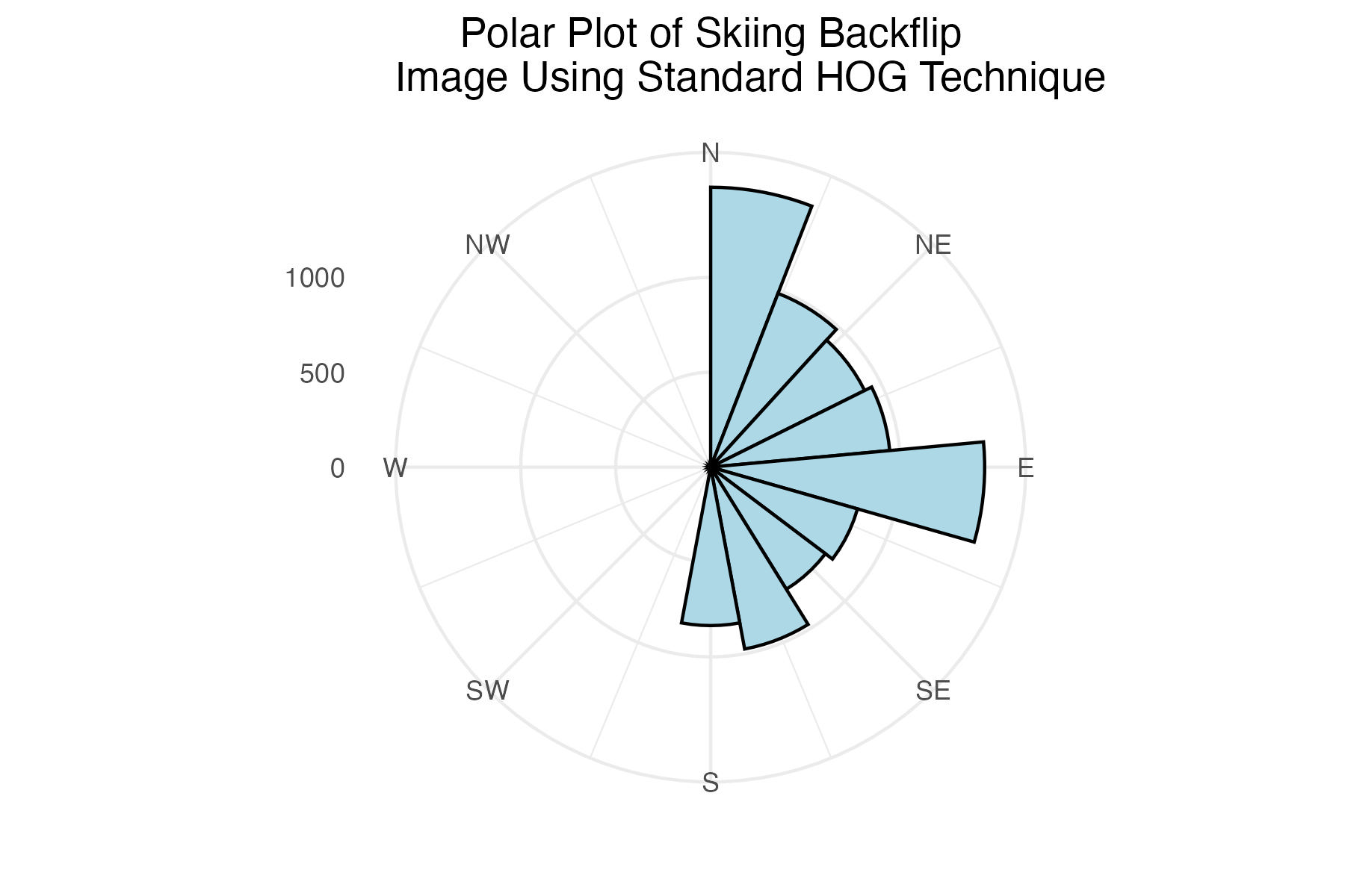
Discussion
When looking at the gradient magnitudes in image form the most definitive lines occur where the snow from the jump is visible. This makes sense, because the snowy jump is a uniform white, resulting in minimal gradient magnitudes from one pixel to the next within this area. When the edge of the snow meets the crowd in the background, there is a great increase in gradient magnitude. Since the snowy jump in this image is mostly horizontal with some incline and decline, both polar plots identify the horizontal angle as being the most frequent. Interestingly, the distributed binning technique has a notably smaller frequency of vertical lines, likely due to the greater influence of magnitudes on their contribution to the histogram.